Testing graph databases
One of the main components of GUAC is a graph database to store all the metadata pertaining to the software supply chain. Although I promised a while back to have a series of articles about security concepts around software development life-cycle this won’t be that article. Here, I only want to focus on the graph databases, testing several for the GUAC usecase. There is an issue to analyze and select a database backend (by default, GUAC architecture allows replacing the backend behind the GraphQL interface, the backend where the metadata is actually stored).
We started GUAC with a Neo4j backend, which we then partially migrated to the GraphQL design. But, there are several issues (including licensing questions) regarding this solution and this requires us to switch to another database. There is a suggestion to use ArangoDB, which is currently work in progress (almost completed by the time this gets published, slightly more than a month after starting the experiments described within).
I am using this article to study various graph database backends, both because these would help GUAC but also because some of my (future/potential) side projects involve graph databases. Thus, the results from here do not imply that GUAC will change to the database backend. Instead this should be taken only as a personal exploration.
Besides the 2 databases mentioned above, I will consider 4 others:
- Cayley: inspired by Google’s graph database, selected as I have been following the repository for several years, when I was last exploring alternatives to Neo4j;
- TerminusDB: wants to be
Git for data
, offering a user experience that would be very similar to using Git. Also interesting to look at since the codebase uses significant amounts of Prolog. - JanusGraph: Part of the Linux Foundation, integrated visualizations, in use by several large companies, main database to play with Gremlin/Tinkerpop.
- NebulaGraph: High speed processing, milliseconds of latency, benchmarked to be the fastest of Neo4j, JanusGraph and itself.
This gives a total of 6 databases to test. But, before doing the actual performance testing, let’s compare these 6 databases across non-functional dimensions, as summarized in the next table (where each database name is a link to the section of this post where the performance analysis and results for that backend is included). Since the post is long, you can see the final conclusion and a summary of all results in this section.
| Database | Development language(s) | Language clients | License | Has Docker | In NixOS | ||
|---|---|---|---|---|---|---|---|
| Go | Python | Haskell | |||||
| Neo4j | Java | ✅ | ✅ | 🟡1 | GPLv3, commercial2 |
✅ | ✅ |
| ArangoDB | C++ | ✅ | ✅ | ❌ | Apache2 | ✅ | ✅ |
| Cayley | Go | ✅ | 🟡3 | 🟡4 | Apache2 | ✅ | ✅ |
| TerminusDB | Prolog/Rust | ❌ | ✅ | ❌ | Apache2 | ✅ | ❌ |
| JanusGraph | Java | 🟡5 | 🟡6 | 🟡7 | Apache2, CC-BY-4.08 |
✅ | 🟡9 |
| NebulaGraph | C++ | ✅ | ✅ | ❌ | Apache2 | ✅ | ❌ |
It seems that the only language that all these databases have a driver for is Python (with some caveats). Haskell support is severely lacking, as the only existing packages are out of date or are very generic. Fortunately, all these databases use Docker (with caveats). As such, the testing scenario will use Python language and connect to the database running in a Docker container. It is possible that in the final projects I’ll use the NixOS deployment directly, but that is out of scope for this post.
Testing scenario 🔗
Since my own personal projects are only at ideas stage – meaning the usecases are not yet clearly defined –, the testing performed in this article will simulate scenarios needed in GUAC. Fortunately, there is some overlap with the incipient ideas I have in mind. In broad lines, we want to ingest packages and dependencies between them. We will use something similar to GUAC’s Package ontology: for each package we need 4 different nodes: one for the type of the ecosystem, one for an optional namespace that the ecosystem might support, one for the name of the package and one for the version. These should match the pURL format for package identifiers, removing the qualifiers and subpath optional fields. For the dependencies, we will only add one additional node linking 2 version nodes, as in the following image:
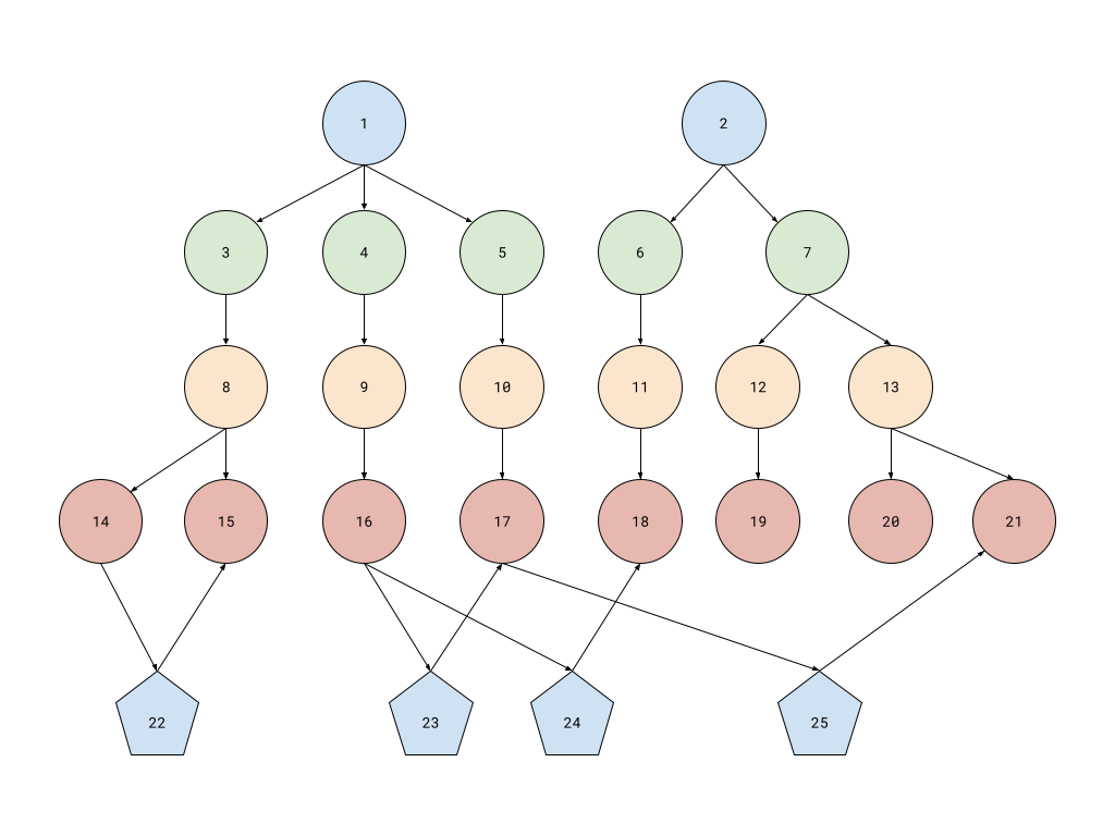
Here, nodes 1 and 2 represent two different ecosystems (e.g., PyPI and
npm). Nodes 3 to 7 represent various namespaces. Nodes 8-13 represent
different package names and nodes 14 to 21 represent various versions of these
packages. Nodes 22 to 25 represent dependency information such as:
- node 22 states that package 14 depends on package 15. These are 2 versions of the same package name, so this is either a bad configuration or some scenario which would require bootstrapping;
- nodes 23 and 24 show two dependencies of package 16, one of which (18) is in the other ecosystem;
- node 25 also records a cross-ecosystem dependency. It also records a transitive dependency chain between 16 and 21 (16 - 23 - 17 - 25 - 21).
Note: this is a simplification of the data model from GUAC, but it should cover the critical parts. This means that the results from here will not translate 100%, but we will still have some ideas about forward paths.
Data generation 🔗
Since I am interested in how these databases scale, I need to be able to ingest a wide range of package. Hence, instead of using real data we’ll have to use fake, synthetic input. This can be done by picking a number \(N\) for the total number of packages to ingest and representing each package by a number \(x\), from \(0\) to \(N-1\). To build the pURL description, we can start writing \(x\) in a base \(B\) (equivalent to a branching factor in the package trie): we have \(x = x_0 + x_1B + x_2B^2 + \ldots\) and from this we can extract the other components that identify the package:
- package ecosystem: node \(x_0\) of the root of the trie
- package namespace: node \(x_1\) of the package ecosystem selected above
- package name: node \(x_2\) of the package namespace selected above
- package version: a new child of the name node selected above, labeled \(x\) (the full package name)
That is, the pURL for a package labeled \(x\) is
pkg:\(x_0\)/\(x_1\)/\(x_2\)@\(x\). This has really interesting properties, as
we will see in a short while.
Moving to the dependencies between these packages, since this is another dimension we need to test scalability on, let’s pick a number \(K\) to denote the maximum number of dependencies each package can have. Then, for a package \(x\), we consider it to depend on the set \(\left\{ \left[\frac{x}{k}\right] \phantom{1}|\phantom{1} k \in \{2, 3, \ldots K + 1\}\right\}\). That is, take all numbers \(k\) from 2 to \(K+1\) (so that there are \(K\) of them), divide \(x\) by \(k\) and record a dependency to the quotient, if one was not already present. For example, package \(100\) can depend on packages \(50, 33, 25, 20, \ldots\) (the first \(K\) of these), whereas package \(2\) can only depend on packages \(1\) and \(0\) (if \(K = 1\) then only on package \(1\)). As \(K\) increases, the connectivity between nodes in the graph increases fast. If \(N\) is large enough, nodes can have up to \(2K + \frac{K(K+1)}{2}\) total dependencies (for example if \(K=3\), node \(x=6\) has 3 dependencies – 1, 2, 3 – and is in the dependency set of 12, 13, 18, 19, 20, 24, 25, 26, and 27). The proof of this statement is left as an exercise to the reader :)
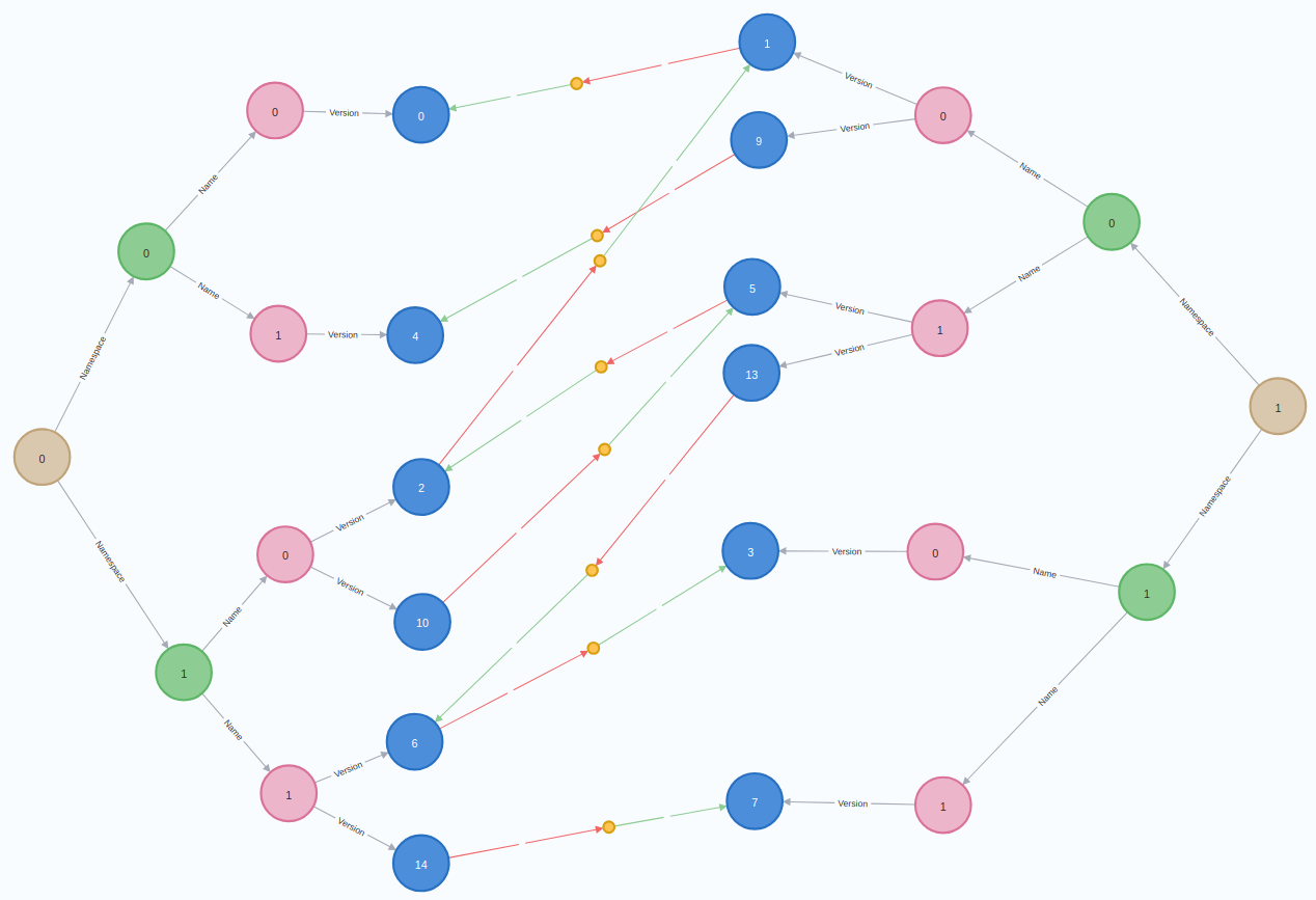
An ingestion scenario is uniquely identified by the 3 numbers, \(N\), \(B\), and \(K\). For example, the following image is the result of ingesting \(N=16\) packages, with a branching factor of \(B=2\) and each package having at most \(K=1\) dependencies:
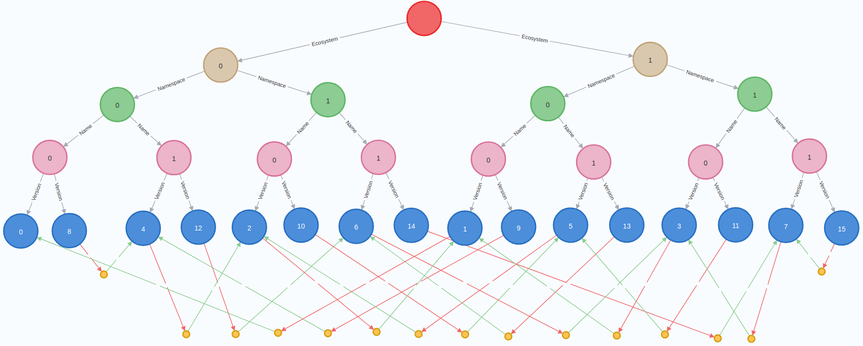
Here, the root of the package trie is the single empty red node, ecosystems are marked by the 2 brown nodes, namespaces by the 4 green ones, package names by the 8 pink ones, packages (i.e., package versions) by the 16 blue ones and dependencies by the small yellow nodes. The dependency information is encoded by a red arrow, followed by a dependency node, followed by a green arrow to the dependency.
This method of generating data brings a few useful properties that can be used to validate that the results of queries/ingestions are valid (this is especially useful when doing ingestion on multiple threads):
- Cross ecosystem dependencies are dependencies where the parent and the dependency packages have different remainders when divided by \(B\). For example, \(14\) and \(7\) have different parity, thus this is a cross ecosystem dependency in the scenario from the picture above.
- Dependencies between versions of the same package (invalid configurations, or recording a need to bootstrap) are dependencies where the parent and the dependency packages have the same values for \(x_0\), \(x_1\) and \(x_2\). That is, they are equal modulo \(B^3\). In the image above, this is the case of packages \(15\) and \(7\) (if we were to use \(K=2\) then we would also have had a similar situation for \(11\) and \(3\)).
It is trivial to prove these properties, so they are left as an exercise to the reader :)
Ingestion tests 🔗
When ingesting the data, there are 2 major scenarios to consider: ingesting only packages (which is in general a write-only query, to add the missing nodes), and ingesting dependencies (which will need to locate existing packages and then add the dependency node between them – we assume, like in GUAC, that each dependency node is created between packages already ingested, as this should simplify the queries on the backend).
Ingesting packages can be done in 2 ways: ingest packages one by one as they are “found” (generated from \(x\)) and ingest packages all at once, in a batch (an extreme case, in general we might want to ingest batches of up to a certain number of packages). That is:
- For each \(x\), ingest package \(x\).
- Collect all packages in a list, ingest the list.
In the first case, we can ingest packages in increasing order or in a random order, to detect cases where the ingestion pattern might be relevant for performance. To simplify testing, all randomness will be generated with a fixed seed randomly selected to be 42.
Ingesting dependencies can be done in 3 different ways: ingest each dependency one by one (in order or shuffled) (by ingesting the 2 packages and then the dependency node), ingest all dependencies of each package individually (in order or shuffled) (by first collecting all dependency packages in a list, batch ingesting the parent package and the list of dependencies and then batch ingesting the dependency nodes), ingesting all dependencies at once in a batch. That is:
- For each \(x\), generate a list of up to \(K\) dependencies. For each dependency in the list, ingest \(x\) and the dependency package and then the dependency node. It is obvious that this results in duplicated effort, as package \(x\) will be attempted to be ingested \(K\) times, but \(K-1\) times it would be present in the database already.
- For each \(x\), generate a list of up to \(K\) dependencies. Then, from this list collect the set of all packages and ingest them all in a batch. When this is done, ingest all dependency nodes in a batch.
- Collect all packages in a list, expand the list to contain all dependencies
(
concatMap). Then, collect all packages and batch ingest them, then batch ingest all dependency nodes.
Thus, there are 5 different scenarios for ingestion. For each on of them we can define some qualifiers:
- ingest in increasing order or ingest in a shuffled order;
- ingest with all relevant indexes present or without any database index;
- ingest in a single thread or in multiple threads.
The last mode is not valid when ingesting everything in a big batch (all packages at once or all dependencies at once) since we’re doing a single database call but with large amount of data.
Between each ingestion experiment the database will be dropped, removing all nodes and indexes.
Query tests 🔗
After we run all ingestion experiments, we’ll perform one more ingestion and then run the following query experiments to test read-only performance:
Find all dependency paths that are within the same package name (i.e., invalid, or requiring bootstrapping). In the graph above, this should return only the set \(\{15, 7\}\).
Find all dependency paths that cross ecosystem boundaries. In the graph above, this is:
\[\{\{14, 7\},\{13, 6\},\{10, 5\},\{9, 4\},\{6, 3\},\{5, 2\},\{2, 1\},\{1, 0\}\}\]
These are testing simple graph patterns and the results have vastly different cardinalities. These queries might easily translate to SQL, but larger path queries might not. However, due to length constraints, I decided to leave more advanced path queries for another article, running them only on a subset of these databases.
Since in general these queries are run by a single user, each will be run in single threaded environment. However, the performance of these queries might still be influenced by the presence of indexes, so we have 2 run modes.
Generic code 🔗
There is a large amount of code that we’ll have to write. First, we can begin with some trivial imports and then define 2 dataclasses to hold packages and dependencies:
import argparse
import concurrent.futures
import math
import random
import requests # optional, needed for some databases
import retry    # optional, needed for some ArangoDB cases
import time     # optional, needed for some databases

from collections import defaultdict
from dataclasses import asdict, dataclass
from datetime import datetime
from typing import Callable, Self, Sequence


@dataclass(frozen=True)
class Package:
    ecosystem: str
    namespace: str
    name: str
    version: str


@dataclass(frozen=True)
class Dependency:
    parent: Package
    target: Package
Now, we can define the general class for an experiment. First, the initialization/construction parts:
class Experiment:
    def __init__(self, N: int, B: int, K: int, shuffle: bool = False,
                 threaded: bool = False):
        self.N = N
        self.B = B
        self.K = K
        self.shuffle = shuffle
        self.threaded = threaded

    def setup(self, indexes: bool = True):
        pass

    #...
In __init__ we pass values for \(N\), \(B\) and \(K\) and also store the
qualifiers for whether the experiment should run on multiple threads, or
shuffle the data before ingestion.
Since each database needs to run specific code during initialization (e.g.,
set up indexes, set up initial structure), I decided to separate that into a
setup function10. For the base base there is nothing to do here.
Next thing to define are 2 helper methods that process a value \(x\) and generate the package pURL or the list of dependencies for the package:
class Experiment:
    #...

    def _generate_package(self, x: int) -> Package:
        version = x
        ecosystem, x = x % self.B, x // self.B
        namespace, x = x % self.B, x // self.B
        name = x % self.B
        return Package(f'{ecosystem}', f'{namespace}', f'{name}', f'{version}')

    def _generate_dependencies(self, x: int) -> Sequence[Dependency]:
        deps = []
        old = x
        parent = self._generate_package(x)
        for k in reversed(range(2, self.K + 2)):
            target = x // k
            if target == old: continue
            target = self._generate_package(target)
            deps.append(Dependency(parent, target))
        return deps

    #...
Since we don’t want to duplicate edges (e.g., for \(x=4\) and \(K=4\), because \([4/3]=1\) and \([4/4]=1\) we would naively draw 2 edges between \(4\) and \(1\)), we generate the dependencies in reverse order and compare with the last ingested dependency.
Looking at the ingestion experiments, there are 2 categories: ones that run in a batch, ingesting everything all at once, and those that ingest one package/dependency one by one. Since we don’t want to duplicate code, let’s define runner functions to take care of timing, shuffling, and adding threading support as needed:
class Experiment:
    #...

    def _experiment(self, work: Callable[int, None], reverse: bool = False):
        start = datetime.now()

        seq = range(self.N)
        if self.shuffle:
            random.seed(42)
            seq = random.sample(seq, self.N)
        elif reverse:
            seq = reversed(seq)

        if self.threaded:
            with concurrent.futures.ThreadPoolExecutor() as executor:
                futures = [executor.submit(work, x) for x in seq]
                for future in concurrent.futures.as_completed(futures):
                    pass # no results to return
        else:
            for x in seq:
                work(x)

        end = datetime.now()
        print(f'Duration: {end - start}')

    def _batch_experiment(self, work: Callable[None, None]):
        start = datetime.now()
        work()
        end = datetime.now()
        print(f'Duration: {end - start}')

    #...
Observe how for batches there is no threading support and no shuffling defined here. Shuffling will be done when creating the work item, but threading is irrelevant since there is only one call to the database backend.
Now, we can define the ingestion experiments. First, the packages:
class Experiment:
    #...

    def ingest_packages(self):
        def work(x):
            self._do_ingest_package(self._generate_package(x))

        self._experiment(work)

    def batch_ingest_packages(self):
        def work():
            pkgs = [self._generate_package(x) for x in range(self.N)]
            if self.shuffle:
                random.seed(42)
                pkgs = random.sample(pkgs, self.N)
            self._do_ingest_batch_packages(pkgs)

        self._batch_experiment(work)

    #...
We’re defining an inner work worker (using a worker-wrapper
pattern from Haskell world) and passing that to the 2
experiment runners. It could be possible to remove the duplication for the
shuffling in batch_ingest_packages, but that refactoring is also left
as an exercise to the reader.
Similarly, we can define the 3 methods to ingest dependencies:
class Experiment:
    #...

    def ingest_dependencies(self):
        def work(x):
            for dependency in self._generate_dependencies(x):
                self._do_ingest_package(dependency.parent)
                self._do_ingest_package(dependency.target)
                self._do_ingest_dependency(dependency)

        self._experiment(work, reverse=True)

    def split_ingest_dependencies(self):
        def work(x):
            deps = self._generate_dependencies(x)
            if not deps: return
            pkgs = [self._generate_package(x)]
            for dependency in deps:
                pkgs.append(dependency.target)
            self._do_ingest_batch_packages(pkgs)
            self._do_ingest_batch_dependencies(deps)

        self._experiment(work, reverse=True)

    def batch_ingest_dependencies(self):
        def work():
            pkgs = [self._generate_package(x) for x in range(self.N)]
            deps = []
            for x in range(self.N):
                deps.extend(self._generate_dependencies(x))
            if self.shuffle:
                random.seed(42)
                pkgs = random.sample(pkgs, len(pkgs))
                deps = random.sample(deps, len(deps))
            self._do_ingest_batch_packages(pkgs)
            self._do_ingest_batch_dependencies(deps)

        self._batch_experiment(work)

    #...
The first method ingests data as it is generated, whereas the other two try to batch it, as discussed in the previous section. Note that the more advanced ingestion methods have been optimized from the naive versions listed below:
class Experiment:
    #...

    def naive_split_ingest_dependencies(self):
        def work(x):
            pkgs = set()
            deps = self._generate_dependencies(x)
            for dependency in deps:
                pkgs.add(dependency.parent)
                pkgs.add(dependency.target)
            if pkgs: self._do_ingest_batch_packages(pkgs)
            if deps: self._do_ingest_batch_dependencies(deps)

        self._experiment(work, reverse=True)

    def naive_batch_ingest_dependencies(self):
        def work():
            deps = set()  # can also be a list -- exercise to the reader :)
            for x in reversed(range(self.N)):
                deps = deps.union(self._generate_dependencies(x))
            pkgs = set()
            for dependency in deps:
                pkgs.add(dependency.parent)
                pkgs.add(dependency.target)
            if self.shuffle:
                random.seed(42)
                pkgs = random.sample(pkgs, len(pkgs))
                deps = random.sample(deps, len(deps))
            if pkgs: self._do_ingest_batch_packages(pkgs)
            if deps: self._do_ingest_batch_dependencies(deps)

        self._batch_experiment(work)

    #...
These versions try to use set operations to remove duplicates (and
under real world scenarios we would have to use these). However, our
experiments will run with very large numbers of batches, making the set
operations be really expensive. The naive versions can be up to 100 times
slower than the optimized ones! Since we know patterns in data (e.g, for split
ingestion we always have the same parent package and each target is a new
package; for batch ingestion we have all packages and all dependencies), we
can remove the need for set operations. This speed gain only affects data
generation, so it wouldn’t pollute the database benchmarks.
Next, let’s write the runners for the read-only queries. Here, I decided to not write a new helper, opting instead for a slightly repeated code:
class Experiment:
    #...

    def query_bootstrap(self):
        start = datetime.now()
        pkgPairs = self._do_query_bootstrap()
        end = datetime.now()
        print(f'Duration: {end - start}')
        valid = True
        B3 = self.B * self.B * self.B
        for parent, target in pkgPairs:
            parent = int(parent)
            target = int(target)
            if parent % B3 != target % B3:
                valid = False
                break
        if valid:
            pairs = set()
            for x in range(self.N):
                for k in range(2, self.K + 2):
                    y = x // k
                    if x == y: continue
                    if x % B3 == y % B3:
                        pairs.add((x, y))
        print(f'Valid: {valid and len(pairs) == len(pkgPairs)}')

    def query_ecosystem(self):
        start = datetime.now()
        pkgPairs = self._do_query_ecosystem()
        end = datetime.now()
        print(f'Duration: {end - start}')
        valid = True
        for parent, target in pkgPairs:
            parent = int(parent)
            target = int(target)
            if parent % self.B == target % self.B:
                valid = False
                break
        if valid:
            pairs = set()
            for x in range(self.N):
                for k in range(2, self.K + 2):
                    y = x // k
                    if x == y: continue
                    if x % self.B != y % self.B:
                        pairs.add((x, y))
        print(f'Valid: {valid and len(pairs) == len(pkgPairs)}')

    #...
In both cases, we only measure the time taken to communicate with the database, and not the verification process. This is because in a real application we will not have a way or a need to validate the query results. This code exists only to validate that the ingestion was successful as we are experimenting with different query patterns. Each validation takes into account the properties we have discovered in previous sections and makes sure that only the valid answers are generated.
In order to control when the database gets cleared (both data and indices), we will also have a worker-wrapper pattern:
class Experiment:
    #...

    def clean(self):
        self._do_clean()

    #...
This is not included as part of __del__ as we want to control when the
dataset gets cleared.
There is one remaining thing to do. We have seen a few helper functions above to perform the actual ingestion/querying, so we need to define them:
class Experiment:
    #...

    def _do_ingest_package(self, package: Package):
        pass

    def _do_ingest_batch_packages(self, packages: Sequence[Package]):
        pass

    def _do_ingest_dependency(self, dependency: Dependency):
        pass

    def _do_ingest_batch_dependencies(self, dependencies: Sequence[Dependency]):
        pass

    def _do_query_bootstrap(self):
        return [] # no data stored

    def _do_query_ecosystem(self):
        return [] # no data stored

    def _do_clean(self):
        pass
These are all empty/trivial. This is because we want each backend to only
implement these (as well as setup, __init__, and __del__
as needed) – this is the strategy design pattern. This also gives
us the benefit that we can measure the time needed to generate the synthetic
data. Thus, we can efficiently measure the time it takes to ingest this data
for each database backend, even in cases where data generation and data
ingestion are interleaved. In the GUAC case, this is almost the difference
between ingesting packages from the guacone command versus ingesting them
from the GraphQL API.
Finally, we need to write the boilerplate needed to set-up all the experiments and run them. I chose to start each experiment from the command line instead of writing a large script as this allows me to inspect the dataset, try various hypotheses, etc. Without further ado, here it is:
backends = {
    'none': Experiment,
    'neo4j': Neo4j,
    'arango': Arango,
    'cayley': Cayley,
    'terminus': TerminusDB,
    'janus': JanusGraph,
    'nebula': NebulaGraph,
}

experiments = {
    'packages': Experiment.ingest_packages,
    'batch_packages': Experiment.batch_ingest_packages,
    'dependencies': Experiment.ingest_dependencies,
    'split_dependencies': Experiment.split_ingest_dependencies,
    'batch_dependencies': Experiment.batch_ingest_dependencies,
    # read queries
    'bootstrap': Experiment.query_bootstrap,
    'ecosystem': Experiment.query_ecosystem,
    # cleanup
    'clean': Experiment.clean,
}

def positive_int(arg:str):
    x = int(arg)
    if x <= 0:
        raise ValueError("Argument must be strictly positive")
    return x

def main():
    parser = argparse.ArgumentParser(description="Benchmark Graph DB impls")
    parser.add_argument('backend', help="Backend to use", choices=backends)
    parser.add_argument('experiment', help="Experiment to run", choices=experiments)
    parser.add_argument('N', type=positive_int, help="Number of packages")
    parser.add_argument('B', type=positive_int, help="Branching factor")
    parser.add_argument('K', type=positive_int, help="Dependencies/package")
    parser.add_argument('-i', '--indexes', action='store_true', help="Create indexes in DB before ingestion")
    parser.add_argument('-s', '--shuffle', action='store_true', help="Shuffle data before ingestion")
    parser.add_argument('-t', '--threaded', action='store_true', help="Use threads to ingest")
    result = parser.parse_args()
    print(result)
    experiment = backends[result.backend](N=result.N, B=result.B, K=result.K,
                                          shuffle=result.shuffle,
                                          threaded=result.threaded)
    experiment.setup(result.indexes)
    experiments[result.experiment](experiment)

if __name__ == '__main__':
    main()
Using argparse makes it easier to specify experiment qualifiers instead
of having to manually pass in True/False arguments if all
experiments were started using only positional arguments. I’m printing the
result of parsing the command line arguments to log each experiment to
a file which I can then process to extract the timing information11.
With this setup done, it is time to start benchmarking. We can benchmark the
none backend to test data generation, and the performance results for
this mode are summarized here. Each database will have its own
section to discuss implementation and then present the benchmark results.
Performance of the databases 🔗
While developing the code for the benchmarks, I used \(N=10\) or \(N=16\), \(B=2\) or \(B=3\), and \(K=1\) up to \(K=4\). But these scenarios are small data, and we cannot extract much significant information from these.
For the experiments, I was planning to run ingestion using \(N=10, N=100,
\ldots, N=1000000\) (1 million) packages. For each of these, I would test with
\(B=2, B=3\), and \(B=10\). Finally, for \(K\) I would use 4 values: \(1, 2, 5\) and
\(10\). Each of these would be run in all the possible modes (all combinations
of passing the -i/-s/-t flags or not). Each experiment would be run 5
times to compute statistical averages.
But we’re not doing that :). We know from the previous article that we need to do some experimental design, since the number of combinations is really large. As described in the previous paragraph, there are 2880 experiments to run. Assuming an upper bound of half an hour for each, this would take a total of 2 months to complete, excluding all the time spent experimenting with different queries, learning the database backends, fixing errors, using the computer for other things12.
Instead, let’s use an alternate strategy. First we’ll try to determine the impact of each of the 3 flags: keeping \(N=10000\), \(B=5\), \(K=5\), we will run each ingestion experiment in 4 settings: no flag set, or exactly one the flags being set. This results in 20 benchmark types.
Similarly, after finishing the ingestion with no flag (or the ingestion with
-i), we will run the 2 queries, thus studying the impact of the index on the
read queries. This brings an additional of 4 benchmark types.
For future benchmark types, since we know the impact of the flags, we will
always run with the combination of -i/-t that gives the most performance.
Next thing to study is the impact of increasing \(N\). We fix \(B=5\), \(K=5\) as before and increase \(N\) by consecutive powers of 10 (\(10, 100, 1000, 10000, 100000, 1000000\)). For each of these values we run all 5 ingestion experiments and the 2 query ones. This adds 35 new benchmark types (since the 10k values are already measured), but we will cut this process short as soon as one ingestion takes more than 30 minutes. For batch ingestion, it is also possible to run out of memory for the driver, so that will also result in a pruning of the search space.
Then, we can study the impact of \(B\). We revert to \(N=10000\) and test the impact of \(B=2\), \(B=4\) and \(B=8\) for both ingestion and querying. This adds 21 more benchmark types.
The value of \(K\) is only relevant when we have dependencies, so we no longer need to study the ingestion of packages by themselves. Let’s use \(N=10000\), \(B=5\) and study \(K=1\), \(K=2\), \(K=4\), \(K=8\). This gives 20 more benchmark types.
In total, we have 100 benchmark types, a significant reduction (6x!) from the entire space of parameters from the start of this section. We’ll run each of them 5 times, setting battery on performance mode (as per the study on battery power mode impact on performance) and having no other user applications opened.
Even with this design, we can collect up to 500 data points. So, instead of presenting the full data, I will only summarize it. This way, the blog post won’t be made artificially long by inclusion of tables with 500 rows.
Note: Between each run for an ingestion benchmark, I’ll drop the database, deleting all indexes that might be present. The database from the last round of ingestion with dependencies will be used for the query benchmarks.
To compute the time taken by database alone (that is, to eliminate time taken to generate the test harness), we can assume that all measurements are normally distributed and then use the fact that the difference of two normal distributions is also a normal distribution.
Finally, note that in some cases there might be multiple possible options to write a query, with different performance implications. If that is the case, I will include a discussion of each, but will include in the final data only the query that seems to be the most performant. I am not an expert in these databases, so I’m leaving open the option for some expert to write the queries to be more efficient, at which point I will update the article as needed.
That’s all, now we can begin the study.
No backend 🔗
We begin first with the baseline that does no database call. There’s nothing to do here: we already discussed the test harness code, so now we only have to present the data tables and graphs:
First experiment is testing the effect of the runtime flags:
| Experiment | type | time (s) | stddev (s) |
|---|---|---|---|
packages |
0.014 | ±0.000 | |
| index | 0.014 | ±0.000 | |
| shuffled | 0.017 | ±0.000 | |
| threads | 0.368 | ±0.179 | |
batch_packages |
0.016 | ±0.001 | |
| index | 0.016 | ±0.000 | |
| shuffled | 0.020 | ±0.000 | |
| threads | 0.016 | ±0.000 | |
dependencies |
0.117 | ±0.001 | |
| index | 0.115 | ±0.002 | |
| shuffled | 0.119 | ±0.001 | |
| threads | 0.724 | ±0.117 | |
split_dependencies |
0.125 | ±0.001 | |
| index | 0.125 | ±0.002 | |
| shuffled | 0.128 | ±0.001 | |
| threads | 0.608 | ±0.073 | |
batch_dependencies |
0.175 | ±0.004 | |
| index | 0.176 | ±0.002 | |
| shuffled | 0.215 | ±0.002 | |
| threads | 0.176 | ±0.004 |
We don’t include the measurements for the time to execute the read queries
since those methods are just pass in the empty implementation.
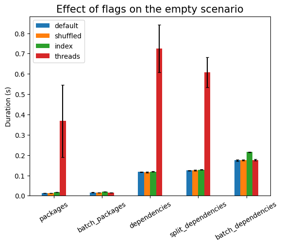
As expected, shuffling the data has to take longer, but there should be no
statistically significant difference between using indexes or not (since there
are no indexes). Using threads is much more expensive here, due to the setup
work needed, except in the cases of batch_*, where there is exactly one
single database call (that is, only one active thread). The setup cost also
explains the large noise in that measurement, compared to the other ones.
Next, we can see the effect of the number of packages, \(N\):
| Experiment | N | time (s) | stddev (s) |
|---|---|---|---|
packages |
10 | 0.003 | ±0.000 |
| 100 | 0.007 | ±0.000 | |
| 1000 | 0.025 | ±0.011 | |
| 10000 | 0.368 | ±0.179 | |
| 100000 | 4.432 | ±0.296 | |
| 1000000 | 51.061 | ±1.867 | |
batch_packages |
10 | 0.000 | ±0.000 |
| 100 | 0.000 | ±0.000 | |
| 1000 | 0.002 | ±0.000 | |
| 10000 | 0.016 | ±0.000 | |
| 100000 | 0.183 | ±0.004 | |
| 1000000 | 2.500 | ±0.081 | |
dependencies |
10 | 0.004 | ±0.000 |
| 100 | 0.009 | ±0.000 | |
| 1000 | 0.038 | ±0.009 | |
| 10000 | 0.724 | ±0.117 | |
| 100000 | 7.033 | ±0.416 | |
| 1000000 | 78.492 | ±1.603 | |
split_dependencies |
10 | 0.004 | ±0.000 |
| 100 | 0.010 | ±0.000 | |
| 1000 | 0.056 | ±0.018 | |
| 10000 | 0.608 | ±0.073 | |
| 100000 | 8.040 | ±0.481 | |
| 1000000 | 83.822 | ±1.920 | |
batch_dependencies |
10 | 0.000 | ±0.000 |
| 100 | 0.002 | ±0.000 | |
| 1000 | 0.016 | ±0.000 | |
| 10000 | 0.176 | ±0.004 | |
| 100000 | 2.597 | ±0.008 | |
| 1000000 | 27.188 | ±0.160 |
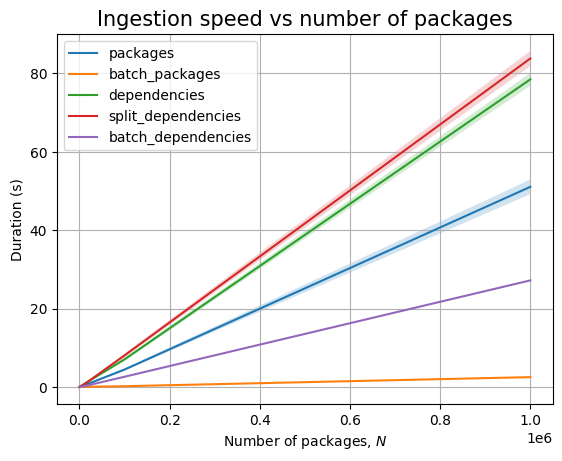
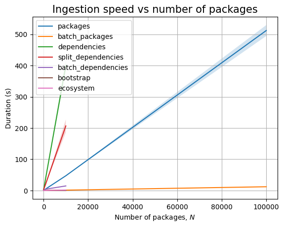
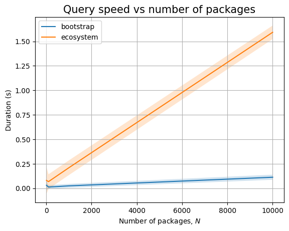
Just like before, time for query execution is 0, since we don’t have a database and we don’t measure the time taken to validate the answers. The timing for the ingestion queries is approximatively linear in \(N\), as can be easily seen when we plot the data:
Next, we can look at the effect of \(B\):
| Experiment | B | time (s) | stddev (s) |
|---|---|---|---|
packages |
2 | 0.470 | ±0.116 |
| 4 | 0.451 | ±0.107 | |
| 8 | 0.436 | ±0.084 | |
batch_packages |
2 | 0.017 | ±0.000 |
| 4 | 0.016 | ±0.000 | |
| 8 | 0.016 | ±0.000 | |
dependencies |
2 | 0.633 | ±0.195 |
| 4 | 0.583 | ±0.063 | |
| 8 | 0.616 | ±0.126 | |
split_dependencies |
2 | 0.657 | ±0.087 |
| 4 | 0.725 | ±0.134 | |
| 8 | 0.627 | ±0.141 | |
batch_dependencies |
2 | 0.174 | ±0.003 |
| 4 | 0.173 | ±0.004 | |
| 8 | 0.173 | ±0.002 |
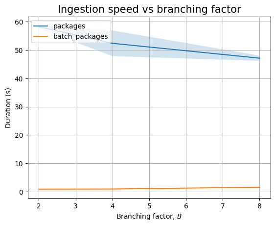
The branching factor \(B\) has no effect in the empty case, as the only thing that changes are the values for the ecosystem, namespace and name fields. We see the similar result when we plot the data:
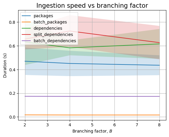
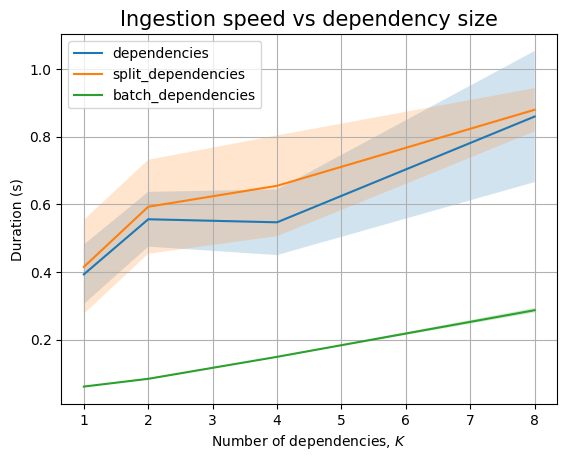
However, we won’t get a similar pattern when looking at the effect of \(K\):
| Experiment | K | time (s) | stddev (s) |
|---|---|---|---|
dependencies |
1 | 0.393 | ±0.088 |
| 2 | 0.556 | ±0.081 | |
| 4 | 0.547 | ±0.097 | |
| 8 | 0.860 | ±0.194 | |
split_dependencies |
1 | 0.415 | ±0.139 |
| 2 | 0.593 | ±0.139 | |
| 4 | 0.655 | ±0.149 | |
| 8 | 0.880 | ±0.064 | |
batch_dependencies |
1 | 0.061 | ±0.001 |
| 2 | 0.084 | ±0.002 | |
| 4 | 0.149 | ±0.001 | |
| 8 | 0.287 | ±0.007 |
Here, the dependency should be linear. And, we see that, in the limit of the noise, when we plot it:
We don’t need to measure anything for the read-only queries, but we will do so on the next sections, when we actually look at database backends.
Neo4j 🔗
For Neo4j, I am using the docker container, started via the following command:
docker run -p 7474:7474 -p 7687:7687 --name neo4j \
  -e NEO4J_AUTH=neo4j/s3cr3tp455 neo4j:latest
Then, for the Python driver, given that I am on Nix, I only need to bring up a shell that contains the corresponding packages:
nix-shell -p python311Packages.neo4jI will use this pattern for the other database backends. This ensures that the
Python environment under which the experiments are run is always clean,
containing only the needed packages, without the need to use venv or similar
sandboxing solutions.
The first thing to do here is to subclass the Experiment class to
create the test suite for Neo4j:
class Neo4j(Experiment):
    def __init__(self, N: int, B: int, K: int, shuffle: bool = True, threaded: bool = True):
        super().__init__(N, B, K, shuffle, threaded)
        import neo4j
        self._driver = neo4j.GraphDatabase.driver(
                "bolt://localhost:7687",
                auth=("neo4j", "s3cr3tp455"))

    def __del__(self):
        self._driver.close()

    #...
This takes care of creating a database connection when an instance of the class is created and removing it when the instance goes out of scope and Python decides to garbage collect it (which is not deterministic).
On the setup function we need to create indexes if the user asks for
them, but there is also a correctness issue that we have to consider. In
Neo4j, we can create new nodes and relationships using CREATE, and we can
pattern match on what is already present using [OPTIONAL] MATCH, but
sometimes we want to create a new entity in a pattern only if it doesn’t
already exist. For example, in our scenario, when ingesting a new package in
the same ecosystem as a previous package, we would prefer to reuse the
existing ecosystem node. Neo4j makes it possible to reuse existing graph
patterns using MERGE: the node/relationship will be created if it doesn’t
already exist. This has an implication, however, when ingesting packages in
multithreaded environments: all of the threads will start ingesting a package
when there is nothing present in the database, so instead of having one single
root node for the trie we could get up to as many as there are cores
available. Fortunately, due to the way MERGE works, having
the root of the trie present in the database when the database is brought up
solves this issue. This is because Neo4j takes locks on all bound existing
entities in a pattern if there are entities that need to be created to
complete the pattern. Thus, this is how we should set up and tear down the
database:
class Neo4j(Experiment):
    #...

    def setup(self, indexes: bool = True):
        def setup_root_node(tx):
            tx.run("MERGE (root:Pkg)")

        with self._driver.session(database='neo4j') as session:
            session.execute_write(setup_root_node)
            if indexes:
                session.run("CREATE INDEX I1 FOR (n:Ecosystem) on (n.ecosystem)")
                session.run("CREATE INDEX I2 FOR (n:Namespace) on (n.namespace)")
                session.run("CREATE INDEX I3 FOR (n:Name) on (n.name)")
                session.run("CREATE INDEX I4 FOR (n:Version) on (n.version)")
                session.run("CALL db.awaitIndexes")

    def _do_clean(self):
        with self._driver.session(database='neo4j') as session:
            session.run("MATCH (n) DETACH DELETE n")
            session.run("DROP INDEX I1 IF EXISTS")
            session.run("DROP INDEX I2 IF EXISTS")
            session.run("DROP INDEX I3 IF EXISTS")
            session.run("DROP INDEX I4 IF EXISTS")
            session.run("CALL db.awaitIndexes")

    #...
We create an index for each type of node that has a scalar property which we
might use in later (sub)queries. We don’t have an index for Dependency
nodes because these don’t have scalar data in this experiment (but do in
GUAC, although even there these are unlikely to be part of a query predicate).
Note that we explicitly pass in the default database name to session(), as
recommended in performance tips page. Over large number of
queries, this should result in a small performance improvement.
Ingesting packages is simple:
class Neo4j(Experiment):
    #...

    def _do_ingest_package(self, package: Package):
        def write(tx):
            query = """
MATCH (root:Pkg)
MERGE (root) -[:Ecosystem]-> (ecosystem:Ecosystem {ecosystem: $ecosystem})
MERGE (ecosystem) -[:Namespace]-> (ns:Namespace {namespace: $namespace})
MERGE (ns) -[:Name]-> (name:Name {name: $name})
MERGE (name) -[:Version]-> (version:Version {version: $version})
"""
            result = tx.run(query, ecosystem=package.ecosystem,
                   namespace=package.namespace, name=package.name,
                   version=package.version)
            return result.consume()

        with self._driver.session(database='neo4j') as session:
            session.execute_write(write)

    #...
We start the query by matching on the singleton Pkg node. Then we use
MERGE patterns to extend from a node to a child in the graph, creating the
child as needed. We don’t use a single MERGE line that connects everything
at once because then Neo4j will create the entire chain (e.g., create a new
set of ecosystem, namespace, name and version nodes even if only the new
version is missing). This is also the reason why we don’t start with MERGE (root:Pkg) -[:Ecosystem]-> ...: if we were to, then the multithread runtime
will create multiple root nodes again. To summarize, we want each MERGE
line to create at most one new bound variable (for the new trie node if it
didn’t already exist).
Note that we MATCH on the root node instead of using MERGE as the first
word in the query. If we use MERGE, this results in one additional operation
during the query execution, as can be seen via profiling.
I’ll discuss profiling in detail a little bit later in this section, but first we want to look at the batch ingestion process code:
class Neo4j(Experiment):
    #...

    def _do_ingest_batch_packages(self, packages: Sequence[Package]):
        def write(tx):
            query = """
UNWIND $packages as pkg
MATCH (root:Pkg)
MERGE (root) -[:Ecosystem]-> (ecosystem:Ecosystem {ecosystem: pkg.ecosystem})
MERGE (ecosystem) -[:Namespace]-> (ns:Namespace {namespace: pkg.namespace})
MERGE (ns) -[:Name]-> (name:Name {name: pkg.name})
MERGE (name) -[:Version]-> (version:Version {version: pkg.version})
"""
            result = tx.run(query, packages=[asdict(p) for p in packages])
            return result.consume()

        with self._driver.session(database='neo4j') as session:
            session.execute_write(write)

    #...
Not much has changed: we just need an additional UNWIND line at the start of
the query to run a loop over the entire batch and then we need to convert the
input from dataclasses to dictionaries.
Next, let’s look at ingesting dependencies too:
class Neo4j(Experiment):
    #...

    def _do_ingest_dependency(self, dependency: Dependency):
        def write(tx):
            query = """
MATCH (root:Pkg)
MATCH (root) -[:Ecosystem]-> (:Ecosystem {ecosystem: $ecosystem1})
             -[:Namespace]-> (:Namespace {namespace: $namespace1})
             -[:Name]-> (:Name {name: $name1})
             -[:Version]-> (v1:Version {version: $version1})
MATCH (root) -[:Ecosystem]-> (:Ecosystem {ecosystem: $ecosystem2})
             -[:Namespace]-> (:Namespace {namespace: $namespace2})
             -[:Name]-> (:Name {name: $name2})
             -[:Version]-> (v2:Version {version: $version2})
MERGE (v1) -[:HasDependency]-> (:Dependency) -[:Dependency]-> (v2)
"""
            result = tx.run(query, ecosystem1=dependency.parent.ecosystem,
                   namespace1=dependency.parent.namespace,
                   name1=dependency.parent.name,
                   version1=dependency.parent.version,
                   ecosystem2=dependency.target.ecosystem,
                   namespace2=dependency.target.namespace,
                   name2=dependency.target.name,
                   version2=dependency.target.version)
            return result.consume()

        with self._driver.session(database='neo4j') as session:
            session.execute_write(write)

    #...
In general, we have to match the 2 pURLs for the two packages. So, even though
in our case the query could just match the version nodes (since the version
contains the full \(x\) for the package), we will write the query assuming the
general case13. We use MATCH statements since we assume that the package
nodes involved in this dependency have been ingested a priori. In this case,
it makes no sense to split the match patterns across multiple statements, each
containing an edge, like we did with MERGE lines when ingesting packages. In
fact, profiling these scenarios show that either query gets compiled to the
same execution tree.
Instead of a MERGE for the dependency node, we could have used CREATE,
since our experiments are only ingesting each dependency once, after which the
dataset is dropped before a new experiment can run. But this won’t translate
to real-world scenario, where multiple documents might record the same
dependency link. Thus we need to make sure we don’t duplicate the dependency
nodes.
Before moving forward, let’s also discuss profiling. It is very simple, all we
have to do is add PROFILE in front of the first word of the query and then
use the result summary object:
        def write(tx):
            query = """
PROFILE ...(rest of query)...
"""
            result = tx.run(query, ...)
            return result.consume()

        with self._driver.session(database='neo4j') as session:
            summary = session.execute_write(write)
            print(summary.profile['args']['string-representation'])
Using profiling, we can see the impact indexes in Neo4j have on the performance of ingesting dependencies. Each summary prints a table with a textual representation of the execution tree for the query and some statistics about the execution. The UI from the web page displays this in a nicer format, but then we’d have to run the query manually. Instead, we’d like to see how query profiling data changes as the database gets populated, if any change occurs.
Turns out, there is actually a change. When not using indexes, we have the following profile, at any point during ingesting dependencies (due to page width constraints, I’m using an inline style to reduce font size and I’m slightly reformatting the output):
+-------------------------------+----+--------------------------------------------+------+------+------+--------+
| Operator                      | Id | Details                                    | Est. | Rows | DB   | Memory |
|                               |    |                                            | Rows |      | Hits | Bytes  |
+-------------------------------+----+--------------------------------------------+------+------+------+--------+
| +ProduceResults               |  0 |                                            |    0 |    0 |    0 |        |
| |                             +----+--------------------------------------------+------+------+------+--------+
| +EmptyResult                  |  1 |                                            |    0 |    0 |    0 |        |
| |                             +----+--------------------------------------------+------+------+------+--------+
| +Apply                        |  2 |                                            |    0 |    1 |    0 |        |
| |\                            +----+--------------------------------------------+------+------+------+--------+
| | +LockingMerge               |  3 | CREATE (anon_15:Dependency),               |    0 |    1 |    5 |        |
| | |                           |    |   (v1)-[anon_14:HasDependency]->(anon_15), |      |      |      |        |
| | |                           |    |   (anon_15)-[anon_16:Dependency]->(v2),    |      |      |      |        |
| | |                           |    | LOCK(v1, v2)                               |      |      |      |        |
| | |                           +----+--------------------------------------------+------+------+------+--------+
| | +Expand(Into)               |  4 | (v1)-[anon_14:HasDependency]->(anon_15)    |    0 |    0 |    0 |    592 |
| | |                           +----+--------------------------------------------+------+------+------+--------+
| | +Filter                     |  5 | anon_15:Dependency                         |    0 |    0 |    0 |        |
| | |                           +----+--------------------------------------------+------+------+------+--------+
| | +Expand(All)                |  6 | (v2)<-[anon_16:Dependency]-(anon_15)       |    0 |    0 |    4 |        |
| | |                           +----+--------------------------------------------+------+------+------+--------+
| | +Argument                   |  7 | v2, v1                                     |    0 |    2 |    0 |        |
| |                             +----+--------------------------------------------+------+------+------+--------+
| +Filter                       |  8 | v2.version = $version2 AND v2:Version      |    0 |    1 |    2 |        |
| |                             +----+--------------------------------------------+------+------+------+--------+
| +Expand(All)                  |  9 | (anon_12)-[anon_13:Version]->(v2)          |    0 |    1 |    3 |        |
| |                             +----+--------------------------------------------+------+------+------+--------+
| +Filter                       | 10 | v1.version = $version1 AND v1:Version      |    0 |    1 |    2 |        |
| |                             +----+--------------------------------------------+------+------+------+--------+
| +Expand(All)                  | 11 | (anon_5)-[anon_6:Version]->(v1)            |    0 |    1 |    3 |        |
| |                             +----+--------------------------------------------+------+------+------+--------+
| +Filter                       | 12 | anon_12.name = $name2 AND anon_12:Name     |    0 |    1 |    3 |        |
| |                             +----+--------------------------------------------+------+------+------+--------+
| +Expand(All)                  | 13 | (anon_10)-[anon_11:Name]->(anon_12)        |    0 |    2 |    4 |        |
| |                             +----+--------------------------------------------+------+------+------+--------+
| +Filter                       | 14 | anon_5.name = $name1 AND anon_5:Name       |    0 |    1 |    3 |        |
| |                             +----+--------------------------------------------+------+------+------+--------+
| +Expand(All)                  | 15 | (anon_3)-[anon_4:Name]->(anon_5)           |    0 |    2 |    4 |        |
| |                             +----+--------------------------------------------+------+------+------+--------+
| +Filter                       | 16 | anon_10.namespace = $namespace2 AND        |    0 |    1 |    2 |        |
| |                             |    | anon_10:Namespace                          |      |      |      |        |
| |                             +----+--------------------------------------------+------+------+------+--------+
| +Expand(All)                  | 17 | (anon_8)-[anon_9:Namespace]->(anon_10)     |    0 |    1 |    3 |        |
| |                             +----+--------------------------------------------+------+------+------+--------+
| +Filter                       | 18 | anon_8.ecosystem = $ecosystem2 AND         |    0 |    1 |    2 |        |
| |                             |    | anon_8:Ecosystem                           |      |      |      |        |
| |                             +----+--------------------------------------------+------+------+------+--------+
| +Expand(All)                  | 19 | (root)-[anon_7:Ecosystem]->(anon_8)        |    0 |    1 |    2 |        |
| |                             +----+--------------------------------------------+------+------+------+--------+
| +Filter                       | 20 | anon_3.namespace = $namespace1 AND         |    0 |    1 |    2 |        |
| |                             |    | anon_3:Namespace                           |      |      |      |        |
| |                             +----+--------------------------------------------+------+------+------+--------+
| +Expand(All)                  | 21 | (anon_1)-[anon_2:Namespace]->(anon_3)      |    0 |    1 |    3 |        |
| |                             +----+--------------------------------------------+------+------+------+--------+
| +Filter                       | 22 | anon_1.ecosystem = $ecosystem1 AND         |    0 |    1 |    3 |        |
| |                             |    | root:Pkg AND anon_1:Ecosystem              |      |      |      |        |
| |                             +----+--------------------------------------------+------+------+------+--------+
| +DirectedRelationshipTypeScan | 23 | (root)-[anon_0:Ecosystem]->(anon_1)        |    3 |    1 |    2 |        |
+-------------------------------+----+--------------------------------------------+------+------+------+--------+
To understand this table, we can find details about each operator on the
operator summary index that Neo4j offers. There
isn’t much to see here. Starting from the root node (operation 23, read the
table from bottom up), Neo4j matches each pattern in order, having very few
rows to return to the operator upwards, very few database hits. This goes
upwards until operator 8, at which point Neo4j has the 2 variables v1 and
v2 for the version nodes that need to be linked into the dependency
structure. Now, it needs to evaluate another branch of the evaluation tree,
where operator 4 finally builds the edge, writing nearly 600 bytes. The edge
is created on operator 3, and we don’t return any result back.
When using indexes, the first few ingestions in the database have the following profile (with similar modifications as above):
+------------------------------+----+--------------------------------------------+------+------+------+--------+
| Operator                     | Id | Details                                    | Est. | Rows | DB   | Memory |
|                              |    |                                            | Rows |      | Hits | Bytes  |
+------------------------------+----+--------------------------------------------+------+------+------+--------+
| +ProduceResults              |  0 |                                            |    0 |    0 |    0 |        |
| |                            +----+--------------------------------------------+------+------+------+--------+
| +EmptyResult                 |  1 |                                            |    0 |    0 |    0 |        |
| |                            +----+--------------------------------------------+------+------+------+--------+
| +Apply                       |  2 |                                            |    0 |    1 |    0 |        |
| |\                           +----+--------------------------------------------+------+------+------+--------+
| | +LockingMerge              |  3 | CREATE (anon_15:Dependency),               |    0 |    1 |    5 |        |
| | |                          |    |   (v1)-[anon_14:HasDependency]->(anon_15), |      |      |      |        |
| | |                          |    |   (anon_15)-[anon_16:Dependency]->(v2),    |      |      |      |        |
| | |                          |    | LOCK(v1, v2)                               |      |      |      |        |
| | |                          +----+--------------------------------------------+------+------+------+--------+
| | +Expand(Into)              |  4 | (v1)-[anon_14:HasDependency]->(anon_15)    |    0 |    0 |    0 |    592 |
| | |                          +----+--------------------------------------------+------+------+------+--------+
| | +Filter                    |  5 | anon_15:Dependency                         |    0 |    0 |    0 |        |
| | |                          +----+--------------------------------------------+------+------+------+--------+
| | +Expand(All)               |  6 | (v2)<-[anon_16:Dependency]-(anon_15)       |    0 |    0 |    4 |        |
| | |                          +----+--------------------------------------------+------+------+------+--------+
| | +Argument                  |  7 | v2, v1                                     |    0 |    2 |    0 |        |
| |                            +----+--------------------------------------------+------+------+------+--------+
| +NodeHashJoin                |  8 | anon_12                                    |    0 |    1 |    0 |    552 |
| |\                           +----+--------------------------------------------+------+------+------+--------+
| | +NodeHashJoin              |  9 | anon_5                                     |    0 |    1 |    0 |    488 |
| | |\                         +----+--------------------------------------------+------+------+------+--------+
| | | +NodeHashJoin            | 10 | anon_10                                    |    0 |    1 |    0 |    624 |
| | | |\                       +----+--------------------------------------------+------+------+------+--------+
| | | | +NodeHashJoin          | 11 | anon_3                                     |    0 |    1 |    0 |    552 |
| | | | |\                     +----+--------------------------------------------+------+------+------+--------+
| | | | | +NodeHashJoin        | 12 | anon_8                                     |    0 |    1 |    0 |    624 |
| | | | | |\                   +----+--------------------------------------------+------+------+------+--------+
| | | | | | +NodeHashJoin      | 13 | root                                       |    0 |    1 |    0 |    568 |
| | | | | | |\                 +----+--------------------------------------------+------+------+------+--------+
| | | | | | | +NodeHashJoin    | 14 | anon_1                                     |    0 |    1 |    0 |    488 |
| | | | | | | |\               +----+--------------------------------------------+------+------+------+--------+
| | | | | | | | +Filter        | 15 | cache[anon_3.namespace] = $namespace1 AND  |    0 |    1 |    2 |        |
| | | | | | | | |              |    | anon_3:Namespace                           |      |      |      |        |
| | | | | | | | |              +----+--------------------------------------------+------+------+------+--------+
| | | | | | | | +Expand(All)   | 16 | (anon_1)-[anon_2:Namespace]->(anon_3)      |    0 |    1 |    3 |        |
| | | | | | | | |              +----+--------------------------------------------+------+------+------+--------+
| | | | | | | | +NodeIndexSeek | 17 | RANGE INDEX anon_1:Ecosystem(ecosystem)    |    0 |    1 |    2 |        |
| | | | | | | |                |    | WHERE ecosystem = $ecosystem1              |      |      |      |        |
| | | | | | | |                +----+--------------------------------------------+------+------+------+--------+
| | | | | | | +Filter          | 18 | root:Pkg                                   |    0 |    1 |    1 |        |
| | | | | | | |                +----+--------------------------------------------+------+------+------+--------+
| | | | | | | +Expand(All)     | 19 | (anon_1)<-[anon_0:Ecosystem]-(root)        |    0 |    1 |    3 |        |
| | | | | | | |                +----+--------------------------------------------+------+------+------+--------+
| | | | | | | +NodeIndexSeek   | 20 | RANGE INDEX anon_1:Ecosystem(ecosystem)    |    0 |    1 |    2 |        |
| | | | | | |                  |    | WHERE ecosystem = $ecosystem1              |      |      |      |        |
| | | | | | |                  +----+--------------------------------------------+------+------+------+--------+
| | | | | | +Filter            | 21 | root:Pkg                                   |    0 |    1 |    1 |        |
| | | | | | |                  +----+--------------------------------------------+------+------+------+--------+
| | | | | | +Expand(All)       | 22 | (anon_8)<-[anon_7:Ecosystem]-(root)        |    0 |    1 |    3 |        |
| | | | | | |                  +----+--------------------------------------------+------+------+------+--------+
| | | | | | +NodeIndexSeek     | 23 | RANGE INDEX anon_8:Ecosystem(ecosystem)    |    0 |    1 |    2 |        |
| | | | | |                    |    | WHERE ecosystem = $ecosystem2,             |      |      |      |        |
| | | | | |                    |    |   cache[anon_8.ecosystem]                  |      |      |      |        |
| | | | | |                    +----+--------------------------------------------+------+------+------+--------+
| | | | | +Filter              | 24 | cache[anon_8.ecosystem] = $ecosystem2 AND  |    0 |    1 |    2 |        |
| | | | | |                    |    | anon_8:Ecosystem                           |      |      |      |        |
| | | | | |                    +----+--------------------------------------------+------+------+------+--------+
| | | | | +Expand(All)         | 25 | (anon_10)<-[anon_9:Namespace]-(anon_8)     |    0 |    1 |    4 |        |
| | | | | |                    +----+--------------------------------------------+------+------+------+--------+
| | | | | +NodeIndexSeek       | 26 | RANGE INDEX anon_10:Namespace(namespace)   |    0 |    1 |    2 |        |
| | | | |                      |    | WHERE namespace = $namespace2,             |      |      |      |        |
| | | | |                      |    |   cache[anon_10.namespace]                 |      |      |      |        |
| | | | |                      +----+--------------------------------------------+------+------+------+--------+
| | | | +Filter                | 27 | cache[anon_3.namespace] = $namespace1 AND  |    0 |    1 |    2 |        |
| | | | |                      |    | anon_3:Namespace                           |      |      |      |        |
| | | | |                      +----+--------------------------------------------+------+------+------+--------+
| | | | +Expand(All)           | 28 | (anon_5)<-[anon_4:Name]-(anon_3)           |    0 |    1 |    3 |        |
| | | | |                      +----+--------------------------------------------+------+------+------+--------+
| | | | +NodeIndexSeek         | 29 | RANGE INDEX anon_5:Name(name)              |    0 |    1 |    2 |        |
| | | |                        |    | WHERE name = $name1                        |      |      |      |        |
| | | |                        +----+--------------------------------------------+------+------+------+--------+
| | | +Filter                  | 30 | cache[anon_10.namespace] = $namespace2 AND |    0 |    1 |    2 |        |
| | | |                        |    | anon_10:Namespace                          |      |      |      |        |
| | | |                        +----+--------------------------------------------+------+------+------+--------+
| | | +Expand(All)             | 31 | (anon_12)<-[anon_11:Name]-(anon_10)        |    0 |    1 |    3 |        |
| | | |                        +----+--------------------------------------------+------+------+------+--------+
| | | +NodeIndexSeek           | 32 | RANGE INDEX anon_12:Name(name)             |    0 |    1 |    2 |        |
| | |                          |    | WHERE name = $name2, cache[anon_12.name]   |      |      |      |        |
| | |                          +----+--------------------------------------------+------+------+------+--------+
| | +Filter                    | 33 | v1.version = $version1 AND v1:Version      |    0 |    1 |    2 |        |
| | |                          +----+--------------------------------------------+------+------+------+--------+
| | +Expand(All)               | 34 | (anon_5)-[anon_6:Version]->(v1)            |    0 |    1 |    3 |        |
| | |                          +----+--------------------------------------------+------+------+------+--------+
| | +NodeIndexSeek             | 35 | RANGE INDEX anon_5:Name(name) WHERE        |    0 |    1 |    2 |        |
| |                            |    | WHERE name = $name1                        |      |      |      |        |
| |                            +----+--------------------------------------------+------+------+------+--------+
| +Filter                      | 36 | cache[anon_12.name] = $name2 AND           |    0 |    1 |    2 |        |
| |                            |    | anon_12:Name                               |      |      |      |        |
| |                            +----+--------------------------------------------+------+------+------+--------+
| +Expand(All)                 | 37 | (v2)<-[anon_13:Version]-(anon_12)          |    0 |    1 |    2 |        |
| |                            +----+--------------------------------------------+------+------+------+--------+
| +NodeIndexSeek               | 38 | RANGE INDEX v2:Version(version)            |    0 |    1 |    2 |        |
|                              |    | WHERE version = $version2                  |      |      |      |        |
+------------------------------+----+--------------------------------------------+------+------+------+--------+
This time we see multiple branches where a range index is used to find a node, and put it in cache. There are several hashed join operations, which are eager (they need to see all of the data from below before producing upstream). This is why these nodes need to reserve memory. In the end, we have a wider but shallower tree.
However, when we get past a certain point in the ingestion process, the profile changes:
+------------------------------+----+--------------------------------------------+------+------+------+--------+
| Operator                     | Id | Details                                    | Est. | Rows | DB   | Memory |
|                              |    |                                            | Rows |      | Hits | Bytes  |
+------------------------------+----+--------------------------------------------+------+------+------+--------+
| +ProduceResults              |  0 |                                            |    0 |    0 |    0 |        |
| |                            +----+--------------------------------------------+------+------+------+--------+
| +EmptyResult                 |  1 |                                            |    0 |    0 |    0 |        |
| |                            +----+--------------------------------------------+------+------+------+--------+
| +Apply                       |  2 |                                            |    0 |    1 |    0 |        |
| |\                           +----+--------------------------------------------+------+------+------+--------+
| | +LockingMerge              |  3 | CREATE (anon_15:Dependency),               |    0 |    1 |    5 |        |
| | |                          |    |   (v1)-[anon_14:HasDependency]->(anon_15), |      |      |      |        |
| | |                          |    |   (anon_15)-[anon_16:Dependency]->(v2),    |      |      |      |        |
| | |                          |    | LOCK(v1, v2)                               |      |      |      |        |
| | |                          +----+--------------------------------------------+------+------+------+--------+
| | +Expand(Into)              |  4 | (v1)-[anon_14:HasDependency]->(anon_15)    |    0 |    0 |    0 |    592 |
| | |                          +----+--------------------------------------------+------+------+------+--------+
| | +Filter                    |  5 | anon_15:Dependency                         |    0 |    0 |    0 |        |
| | |                          +----+--------------------------------------------+------+------+------+--------+
| | +Expand(All)               |  6 | (v2)<-[anon_16:Dependency]-(anon_15)       |    0 |    0 |    4 |        |
| | |                          +----+--------------------------------------------+------+------+------+--------+
| | +Argument                  |  7 | v2, v1                                     |    0 |    2 |    0 |        |
| |                            +----+--------------------------------------------+------+------+------+--------+
| +Filter                      |  8 | v2.version = $version2 AND v2:Version      |    0 |    1 |  126 |        |
| |                            +----+--------------------------------------------+------+------+------+--------+
| +Expand(All)                 |  9 | (anon_12)-[anon_13:Version]->(v2)          |    0 |  125 |  128 |        |
| |                            +----+--------------------------------------------+------+------+------+--------+
| +Filter                      | 10 | v1.version = $version1 AND v1:Version      |    0 |    1 |  126 |        |
| |                            +----+--------------------------------------------+------+------+------+--------+
| +Expand(All)                 | 11 | (anon_5)-[anon_6:Version]->(v1)            |    0 |  125 |  128 |        |
| |                            +----+--------------------------------------------+------+------+------+--------+
| +Filter                      | 12 | anon_12.name = $name2 AND anon_12:Name     |    0 |    1 |    3 |        |
| |                            +----+--------------------------------------------+------+------+------+--------+
| +Expand(All)                 | 13 | (anon_10)-[anon_11:Name]->(anon_12)        |    0 |    2 |    4 |        |
| |                            +----+--------------------------------------------+------+------+------+--------+
| +Filter                      | 14 | anon_5.name = $name1 AND anon_5:Name       |    0 |    1 |    3 |        |
| |                            +----+--------------------------------------------+------+------+------+--------+
| +Expand(All)                 | 15 | (anon_3)-[anon_4:Name]->(anon_5)           |    0 |    2 |    4 |        |
| |                            +----+--------------------------------------------+------+------+------+--------+
| +Filter                      | 16 | anon_10.namespace = $namespace2 AND        |    0 |    1 |    3 |        |
| |                            |    | anon_10:Namespace                          |      |      |      |        |
| |                            +----+--------------------------------------------+------+------+------+--------+
| +Expand(All)                 | 17 | (anon_8)-[anon_9:Namespace]->(anon_10)     |    0 |    2 |    4 |        |
| |                            +----+--------------------------------------------+------+------+------+--------+
| +Filter                      | 18 | anon_3.namespace = $namespace1 AND         |    0 |    1 |    3 |        |
| |                            |    | anon_3:Namespace                           |      |      |      |        |
| |                            +----+--------------------------------------------+------+------+------+--------+
| +Expand(All)                 | 19 | (anon_1)-[anon_2:Namespace]->(anon_3)      |    0 |    2 |    4 |        |
| |                            +----+--------------------------------------------+------+------+------+--------+
| +Filter                      | 22 | root:Pkg                                   |    0 |    1 |    1 |        |
| |                            +----+--------------------------------------------+------+------+------+--------+
| +Expand(All)                 | 23 | (anon_1)<-[anon_0:Ecosystem]-(root)        |    0 |    1 |    4 |        |
| |                            +----+--------------------------------------------+------+------+------+--------+
| +NodeIndexSeek               | 24 | RANGE INDEX anon_1:Ecosystem(ecosystem)    |    1 |    1 |    2 |        |
|                              |    | WHERE ecosystem = $ecosystem1              |      |      |      |        |
+------------------------------+----+--------------------------------------------+------+------+------+--------+
This looks almost similar to the case when no index is being used! But, on a careful read, we see that actually this execution starts from the index of an ecosystem node, instead of scanning all relationships between root and ecosystems. Since these profiles were obtained with \(B = 2\), there is not much difference to see between the cases. We do see some difference on operations 8-11, which are due to the large number of versions (\(N=1000\) means each package name has an average of \(\frac{N}{B^3} \approx 127\) versions). The query analyzer identified that most indexes are useless for this scenario! This happens even when using \(B=10\), once the number of accesses to the databases using the plan that uses all indexes grows above a certain threshold, the optimizer switches to the new one.
Let’s move on. The next item to implement is batch ingestion of dependencies.
Just like batch ingestion of packages, this is trivial: just add the UNWIND
prefix and do the mechanical transformations:
class Neo4j(Experiment):
    #...

    def _do_ingest_batch_dependencies(self, dependencies: Sequence[Dependency]):
        def write(tx):
            query = """
UNWIND $dependencies as dep
MATCH (root:Pkg)
MATCH (root) -[:Ecosystem]-> (:Ecosystem {ecosystem: dep.parent.ecosystem})
             -[:Namespace]-> (:Namespace {namespace: dep.parent.namespace})
             -[:Name]-> (:Name {name: dep.parent.name})
             -[:Version]-> (v1:Version {version: dep.parent.version})
MATCH (root) -[:Ecosystem]-> (:Ecosystem {ecosystem: dep.target.ecosystem})
             -[:Namespace]-> (:Namespace {namespace: dep.target.namespace})
             -[:Name]-> (:Name {name: dep.target.name})
             -[:Version]-> (v2:Version {version: dep.target.version})
MERGE (v1) -[:HasDependency]-> (:Dependency) -[:Dependency]-> (v2)
"""
            result = tx.run(query, dependencies=[asdict(d) for d in dependencies])
            return result.consume()

        with self._driver.session(database='neo4j') as session:
            session.execute_write(write)

    #...
Neo4j supports nested dictionaries, so the transformations are trivial.
It is time to move to read-only queries. Here, instead of returning the entire pURL of a package, we will only return the version node (that is, the value \(x\)). In GUAC the queries are slightly longer as we want to return the full trie path to fill the GraphQL result. There is a possibility to retrieve the version node and then run a separate query to retrieve the pURL. Benchmarking which of the two is faster is out of scope for this article, but might be considered in a follow-up.
For packages needing bootstrap (or invalid dependencies on the same package), we just need to identify diamond patterns like:
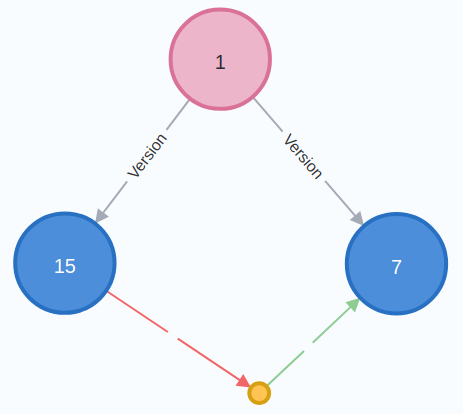
This pattern is easily representable in a query:
class Neo4j(Experiment):
    #...

    def _do_query_bootstrap(self):
        def read(tx):
            pairs = []
            query = """
MATCH (a:Version) <-[:Version]- (:Name) -[:Version]-> (b:Version)
                  -[:HasDependency]-> (:Dependency) -[:Dependency]-> (a)
RETURN b.version AS parent, a.version AS target
"""
            result = tx.run(query)
            for record in result:
                pairs.append((record['parent'], record['target']))
            return pairs

        with self._driver.session(database='neo4j') as session:
            result = session.execute_read(read)
        return result

    #...
Since the read queries return results, profiling is slightly different:
        def read(tx):
            query = """
PROFILE ...(rest of query)...
"""
            result = tx.run(query)
            # process the result
            # return result.consume() for the summary
            return data, result.consume()

        with self._driver.session(database='neo4j') as session:
            result, summary = session.execute_read(read)
            print(summary.profile['args']['string-representation'])
Finding packages that cross ecosystems is also easy once we look at the graph pattern:
We need to match on 2 ecosystem nodes, check that they are different, then expand to version and dependency nodes:
class Neo4j(Experiment):
    #...

    def _do_query_ecosystem(self):
        def read(tx):
            pairs = []
            query = """
MATCH (e1:Ecosystem)
MATCH (e2:Ecosystem)
WHERE e1.ecosystem <> e2.ecosystem
MATCH (e1) -[:Namespace]-> (:Namespace) -[:Name]-> (:Name) -[:Version]-> (v1:Version)
MATCH (e2) -[:Namespace]-> (:Namespace) -[:Name]-> (:Name) -[:Version]-> (v2:Version)
MATCH (v1) -[:HasDependency]-> (:Dependency) -[:Dependency]-> (v2)
RETURN v1.version AS parent, v2.version AS target
"""
            result = tx.run(query)
            for record in result:
                pairs.append((record['parent'], record['target']))
            return pairs

        with self._driver.session(database='neo4j') as session:
            result = session.execute_read(read)
        return result
We already know that we can combine the 3 MATCH lines into a single one,
with a wider pattern and no performance implication:
            query = """
MATCH (e1:Ecosystem)
MATCH (e2:Ecosystem)
WHERE e1.ecosystem <> e2.ecosystem
MATCH (e1) -[:Namespace]-> (:Namespace) -[:Name]-> (:Name) -[:Version]->
      (v1:Version) -[:HasDependency]-> (:Dependency) -[:Dependency]-> (v2:Version)
      <-[:Version]- (:Name) <-[:Name]- (:Namespace) <-[:Namespace]-(e2)
RETURN v1.version AS parent, v2.version AS target
"""
Turns out that it is possible to include the ecosystem matching in the same pattern, without any significant difference in profiling:
            query = """
PROFILE MATCH (e1:Ecosystem) -[:Namespace]-> (:Namespace)
                     -[:Name]-> (:Name)
                     -[:Version]-> (v1:Version)
                     -[:HasDependency]-> () -[:Dependency]-> (v2:Version)
                     <-[:Version]- (:Name)
                     <-[:Name]- (:Namespace)
                     <-[:Namespace]-(e2:Ecosystem)
WHERE e1.ecosystem <> e2.ecosystem
RETURN v1.version AS parent, v2.version AS target
"""
We’ll use the first version as it looks the most readable of all, at no performance cost.
Before continuing to the benchmarking results, I’d like to say that the Python driver for Neo4j has support for custom presentation formats for the query data, so that users of the library don’t need to replicate the same code. In a future article when looking at path queries, I might decide to use these.
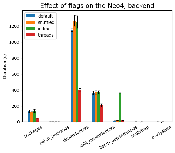
And now, it is time to look at the results:
| Experiment | type | time (s) | stddev (s) |
|---|---|---|---|
packages |
134.540 | ±14.692 | |
| shuffled | 125.821 | ±0.549 | |
| threads | 47.136 | ±0.259 | |
| index | 138.285 | ±19.998 | |
batch_packages |
1.189 | ±0.239 | |
| shuffled | 1.014 | ±0.038 | |
| threads | 1.041 | ±0.044 | |
| index | 1.260 | ±0.100 | |
dependencies |
1149.795 | ±16.339 | |
| shuffled | 1266.392 | ±65.738 | |
| threads | 399.951 | ±17.468 | |
| index | 1251.333 | ±77.973 | |
split_dependencies |
362.864 | ±21.274 | |
| shuffled | 368.909 | ±30.491 | |
| threads | 206.702 | ±20.790 | |
| index | 372.788 | ±19.062 | |
batch_dependencies |
14.635 | ±0.209 | |
| shuffled | 15.409 | ±0.140 | |
| threads | 15.594 | ±0.128 | |
| index | 365.816 | ±6.122 | |
bootstrap |
0.123 | ±0.032 | |
| index | 0.113 | ±0.026 | |
ecosystem |
1.475 | ±0.037 | |
| index | 1.593 | ±0.069 |
We see some surprising effects here. Using indexes does not work well when we
do batch ingestion. The biggest difference is visible in the case of
batch_dependencies, as can be seen in the following plot:
This is explained by the fact that there is work to ensure consistency of the indexes that needs to be done, and in some ingestion scenarios it is better to drop the index, do the bulk ingestion, and then index again. I might run such experiments in a future article, but for now (since data is already generated by the time I’m writing on these sections) we’ll continue with this data.
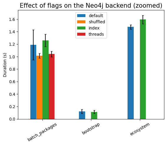
Note, though, that the index is not very effective in increasing the performance of the read queries, as can be seen when we zoom to the corresponding columns:
Next, we need to look at the performance of ingestion when the number of packages increases:
| Experiment | N | time (s) | stddev (s) |
|---|---|---|---|
packages |
10 | 0.280 | ±0.041 |
| 100 | 0.806 | ±0.026 | |
| 1000 | 5.148 | ±0.190 | |
| 10000 | 47.136 | ±0.259 | |
| 100000 | 512.069 | ±17.396 | |
batch_packages |
10 | 0.097 | ±0.018 |
| 100 | 0.086 | ±0.009 | |
| 1000 | 0.184 | ±0.008 | |
| 10000 | 1.189 | ±0.239 | |
| 100000 | 12.026 | ±0.100 | |
dependencies |
10 | 0.878 | ±0.087 |
| 100 | 4.938 | ±0.079 | |
| 1000 | 41.392 | ±0.686 | |
| 10000 | 399.951 | ±17.468 | |
split_dependencies |
10 | 1.726 | ±0.212 |
| 100 | 4.344 | ±0.960 | |
| 1000 | 21.761 | ±0.553 | |
| 10000 | 206.702 | ±20.790 | |
batch_dependencies |
10 | 0.335 | ±0.034 |
| 100 | 0.561 | ±0.035 | |
| 1000 | 4.283 | ±0.032 | |
| 10000 | 14.635 | ±0.209 | |
bootstrap |
10 | 0.031 | ±0.045 |
| 100 | 0.013 | ±0.019 | |
| 1000 | 0.025 | ±0.020 | |
| 10000 | 0.113 | ±0.026 | |
ecosystem |
10 | 0.081 | ±0.138 |
| 100 | 0.068 | ±0.075 | |
| 1000 | 0.210 | ±0.075 | |
| 10000 | 1.593 | ±0.069 |
We are unable to ingest more than 100k packages within the limits imposed. In fact, for dependencies, we cannot even go above 10k!
Increasing \(N\) makes JVM throw out of memory errors when ingesting batches above 100k packages.
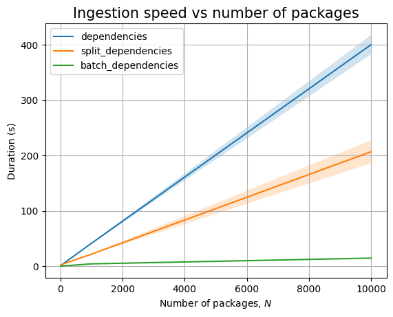
We cannot ingest 100k dependencies in at most 30 minutes, the slope of the ingestion timing graph is significantly high:
Thus, we can only run the read queries up to 10k packages, although we are able to ingest 100k packages. Because we don’t get dependency data for the remaining 90k packages, we won’t run queries above 10k:
The bootstrap patterns are simple, involving only 4 nodes. So the query is running very fast. The query that compares across ecosystem nodes is slow, even in the presence of indexes. This is probably because we still end up traversing large parts of the graph.
In any case, both ingestion and querying look to be linear in the database size.
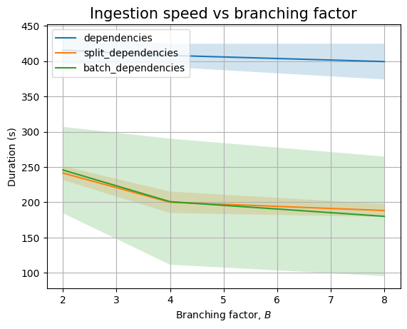
Looking at the branching factor, it looks like there is some complicated relationship between ingestion time and \(B\):
| Experiment | B | time (s) | stddev (s) |
|---|---|---|---|
packages |
2 | 58.210 | ±0.614 |
| 4 | 52.356 | ±4.521 | |
| 8 | 47.117 | ±0.924 | |
batch_packages |
2 | 0.930 | ±0.196 |
| 4 | 0.975 | ±0.021 | |
| 8 | 1.612 | ±0.008 | |
dependencies |
2 | 415.614 | ±19.497 |
| 4 | 408.086 | ±16.535 | |
| 8 | 399.377 | ±25.351 | |
split_dependencies |
2 | 241.499 | ±9.845 |
| 4 | 200.106 | ±15.192 | |
| 8 | 188.399 | ±9.147 | |
batch_dependencies |
2 | 245.788 | ±61.115 |
| 4 | 200.918 | ±89.303 | |
| 8 | 180.162 | ±84.715 | |
bootstrap |
2 | 0.340 | ±0.014 |
| 4 | 0.104 | ±0.008 | |
| 8 | 0.095 | ±0.008 | |
ecosystem |
2 | 1.010 | ±0.074 |
| 4 | 1.455 | ±0.063 | |
| 8 | 1.743 | ±0.061 |
If we look at packages only we see that batch ingestion increases with \(B\), whereas ingesting packages one by one results in a decrease in the ingestion time, even including the measurement noise. As \(B\) increases while \(N\) is kept constant, there are fewer internal nodes that already exist when ingesting new packages, so there is less locking that needs to happen:
If we look at dependencies only we see a similar decreasing trend, though mostly hidden by the noise:
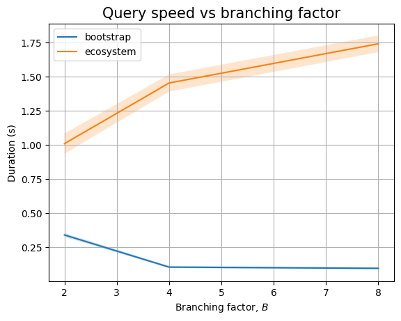
And, if we zoom in to the queries we see two different trends. Queries that only look at package names seem to perform in near constant time (assuming \(B=2\) measurement is severely impacted by biased noise), whereas queries that need to look at internal nodes will have an increasing trend. This could be explained by the fact that there are more edges to look at (proportional to \(B\)):
Next, we can look at \(K\):
| Experiment | K | time (s) | stddev (s) |
|---|---|---|---|
dependencies |
1 | 127.698 | ±1.517 |
| 2 | 203.142 | ±2.851 | |
| 4 | 344.805 | ±14.108 | |
| 8 | 599.730 | ±22.192 | |
split_dependencies |
1 | 107.059 | ±0.750 |
| 2 | 130.092 | ±0.700 | |
| 4 | 186.104 | ±12.937 | |
| 8 | 273.566 | ±10.372 | |
batch_dependencies |
1 | 46.523 | ±0.347 |
| 2 | 90.909 | ±0.941 | |
| 4 | 149.556 | ±68.593 | |
| 8 | 233.779 | ±169.574 | |
bootstrap |
1 | 0.413 | ±0.040 |
| 2 | 0.757 | ±0.017 | |
| 4 | 1.463 | ±0.020 | |
| 8 | 2.886 | ±0.024 | |
ecosystem |
1 | 0.086 | ±0.051 |
| 2 | 0.138 | ±0.055 | |
| 4 | 0.262 | ±0.050 | |
| 8 | 0.476 | ±0.055 |
As expected, ingestion time increases linear with \(K\):
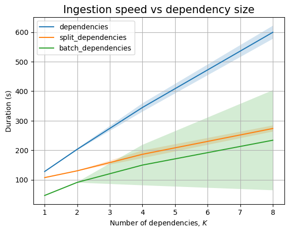
The same pattern occurs in the read queries:
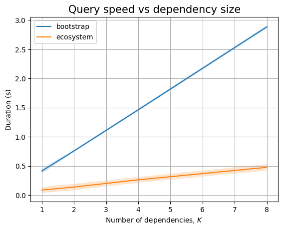
One final note on Neo4j is that these measurements are largely affected by noise, especially at large values of \(N\), \(B\), or \(K\). This seems to be due to the JVM: garbage collection cycles are unpredictable and can stall communication with the database. It might be possible to make them more predictable, but that is out of scope for now.
It is time to look at the new database that GUAC is migrating to.
ArangoDB 🔗
Just like in the Neo4j case, we will use a docker image for the database, which we will start with
docker run -p 8529:8529 --name arango \
  -e ARANGO_ROOT_PASSWORD=s3cr3tp455 arangodb/arangodb:latest
Similarly, we obtain the Python driver via:
nix-shell -p python311Packages.python-arangoArangoDB is a document store database: all data
is stored in the form of JSON objects called documents. These documents may
be organized into collections (documents with the same schema, with
possibility of validating the schema at a cost of minor performance hit).
Collections can be grouped into databases (with a special _system database
that contains internal metadata). Since we don’t want to pollute the special
database, we will create a new one for the experiments. This makes it easy to
drop the database and indexes when the experiment finishes, so it is a win.
Queries in ArangoDB may only touch a single database, but each collection
might have different access controls. Collections can be individually locked,
if needed, and queries are not allowed to read and write to the same
collection in separate statements (thus, if we want to ingest data and then
retrieve it for further ingestion we have to either use special UPSERT
operators or write two separate queries – more on this shortly). In fact,
most AQL (the query language used by ArangoDB) constructs are
not allowed to operate on the same collection in the same query. Each
collection can have various indexes attached to it, but in general only one
index will be used in a query for each collection (the exception only occurs
when FILTER statements use OR to group expressions – but not AND!).
The graph database support for ArangoDB starts by separating collections into two separate types: vertex collections (for nodes) and edge collections (for edges in the graph). The Python API driver uses edge definitions to define these at the same time but leaves open the possibility to define orphan collections for vertex collections that are not included in any edge definitions (which is not the case for us).
With the advent of graph database support in ArangoDB, we now have the ability to either operate directly on the collections (as an anonymous graph) or group them in a named graph. The advantage of a named graph is that it can be displayed in the UI (as in the following image), and that ArangoDB validates that the graph is consistent when data is mutated. This validation might result in performance slowdown, but my testing did not reveal this to be significant. Thus, we will operate on a named graph.
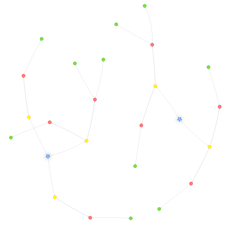
Since each collection should contain documents of similar entities, we will create collections for the 5 node types: ecosystem, namespace, name, version and dependency. We don’t create a special collection for the root of the package trie, since that is a singleton and can be generated when presenting the data to the user (this is unlike Neo4j, there we needed to create the root node to ensure that data is not accidentally duplicated during ingestion; here we will solve this issue in a different way, as will be revealed shortly).
ArangoDB models documents as having 2 separate unique
identifiers: _key (which uniquely identifies a document within its
collection) and _id (which uniquely identifies a document across the
database). Users can provide a custom _key value, or key generators can be
set up when creating collections. The _id field is always automatically
generated based on _key. There is also a _rev
field to implement MVCC-based concurrency, but we won’t make use of
it. Important to remember is that _id and _key are automatically
indexed in indexes that cannot be deleted! These indexes
will be used by ArangoDB by default if there are no other indexes that would
be more efficient for the query, based on the query optimizer.
Edge collections have two additional fields, _from and _to, which also
have specific indexes created for them by default. These fields permit
controlling the traversal direction: inbound (looking at _from),
outbound (looking at _to) or any. Users can create indexes that contains
the _from/_to values in addition to other edge fields to create vertex
specific indexes if edges of multiple types are in the
same collection.
For edges, we can create a single collection for all edges since all these
documents have a similar schema (a key _key, a source _from and a target
_to). But this would harm readability. Furthermore, there is no performance
gain from this. Hence, we will create 5 different edge collections. This also
means that our edges don’t have additional fields, so the vertex specific
indexes will not be useful.
With the considerations so far, we can now write the code to setup and tear down the database under test:
class Arango(Experiment):
    def __init__(self, N: int, B: int, K: int, shuffle: bool = True, threaded: bool = True):
        super().__init__(N, B, K, shuffle, threaded)
        import arango
        self._client = arango.ArangoClient(hosts='http://localhost:8529')

    def __del__(self):
        self._client.close()

    def setup(self, indexes: bool = True):
        self._db_name = "test"
        sys_db = self._select_system_db()
        if not sys_db.has_database(self._db_name):
            sys_db.create_database(self._db_name)
        self._db = self._select_db(self._db_name)

        self._graph_name = "g"
        if self._db.has_graph(self._graph_name):
            self._graph = self._db.graph(self._graph_name)
        else:
            edges = [
                ("ecosystem", "namespace"),
                ("namespace", "name"),
                ("name", "version"),
                ("version", "dependency"),
                ("dependency", "version"),
            ]
            edge_definitions = []
            for src, dst in edges:
                edge_definitions.append({
                    'edge_collection': f'{src}_{dst}',
                    'from_vertex_collections': [src],
                    'to_vertex_collections': [dst]})
            self._graph = self._db.create_graph(
                    self._graph_name, edge_definitions=edge_definitions)

            if indexes:
                pass # No index needed!

    def _do_clean(self):
        sys_db = self._select_system_db()
        sys_db.delete_database(self._db_name)

    def _select_db(self, name: str = "test"):
        return self._client.db(name, username="root", password="s3cr3tp455")

    def _select_system_db(self):
        return self._select_db("_system")

    #...
As discussed, we will used a named graph in setup, but we can replace
all of the corresponding block with the following to create an anonymous one:
        #...

        edges = [
            ("ecosystem", "namespace"),
            ("namespace", "name"),
            ("name", "version"),
            ("version", "dependency"),
            ("dependency", "version"),
        ]
        for src, dst in edges:
            if not self._db.has_collection(src):
                self._db.create_collection(src)
            edge_collection = f'{src}_{dst}'
            if not self._db.has_collection(edge_collection):
                self._db.create_collection(edge_collection, edge=True)

        #...
Similarly, as discussed, we create one edge collection for each type of edge. We generate these based on the name of the two endpoints.
Since we are creating a custom database but we need to access the _system
one for meta-operations, there are 2 helpers, _select_db and
_select_system_db, to ensure that all commands are operating on the
corresponding database.
The last block of setup is supposed to define the indexes that are
relevant for this experiment, to speed up ingestion and querying. But, it
turns out we won’t need any, as will become relevant shortly.
Continuing to package ingestion, we must note that the Python driver has ORM wrappers around ArangoDB operations (among other utilities such as allowing batch, async, and transaction based workflows). This way, we wouldn’t need to write queries manually. However, this won’t translate to other language drivers, so we will use the query language instead (this is also more powerful, allowing us to write queries that retrieve only the data we care about, in patterns that are not easily expressed using OOP constructs).
When ingesting packages in Neo4j we have used MERGE to reuse the prefix of
the trie that has been already ingested and only ingest nodes that were
missing. The equivalent operation here is to use UPSERT (update or insert),
such as the following function:
class Arango(Experiment):
    #...

    @retry.retry()
    def _do_ingest_package_upsert(self, package: Package):
        query = """
LET ecosystem = FIRST(
    UPSERT { ecosystem: @ecosystem }
    INSERT { ecosystem: @ecosystem }
    UPDATE { }
    IN ecosystem
    RETURN NEW)

LET namespace = FIRST(
    UPSERT { namespace: @namespace, parent: ecosystem._key }
    INSERT { namespace: @namespace, parent: ecosystem._key }
    UPDATE { }
    IN namespace
    RETURN NEW)

LET name = FIRST(
    UPSERT { name: @name, parent: namespace._key }
    INSERT { name: @name, parent: namespace._key }
    UPDATE { }
    IN name
    RETURN NEW)

LET version = FIRST(
    UPSERT { version: @version, parent: name._key }
    INSERT { version: @version, parent: name._key }
    UPDATE { }
    IN version
    RETURN NEW)

INSERT {
    _key: CONCAT("e", ecosystem._key, "_", namespace._key),
    _from: ecosystem._id,
    _to: namespace._id,
} INTO ecosystem_namespace OPTIONS { overwriteMode: "ignore" }

INSERT {
    _key: CONCAT("e", namespace._key, "_", name._key),
    _from: namespace._id,
    _to: name._id,
} INTO namespace_name OPTIONS { overwriteMode: "ignore" }

INSERT {
    _key: CONCAT("e", name._key, "_", version._key),
    _from: name._id,
    _to: version._id,
} INTO name_version OPTIONS { overwriteMode: "ignore" }
"""
        variables = {
                'ecosystem': package.ecosystem,
                'namespace': package.namespace,
                'name': package.name,
                'version': package.version,
        }
        self._db.aql.execute(query, bind_vars=variables)

    #...
First, we note that the query is very verbose compared to Neo4j. We have to
run subqueries to build each document type and obtain its node which will then
be used in the edge insertion. For each node, we use UPSERT-INSERT-UPDATE
pattern, where the UPDATE part is empty but the UPSERT and INSERT ones
are identical. If the node we search for with the attributes in UPSERT is
not found, we need to add those attributes as ArangoDB does not add them for
us (compared to Neo4j which allows us to control additional fields using ON CREATE/ON UPDATE)!
Next, note how we had to refer to the parent of each trie node using the
parent field. This is because we would not obtain a trie if we only use the
local fields, since nodes of the same type are placed in the same collection
(that is, ArangoDB is mainly a document store). For example, when ingesting
two namespace nodes from different ecosystem but the same value for
@namespace, if we don’t key on the ecosystem then we would only obtain a
single node.
For the root ecosystem nodes, we need to take into account that UPSERT is
not atomic (unlike MERGE in Neo4j which takes a lock on all bound nodes).
This means that two concurrent write operations might both see that a specific
ecosystem does not exist, create and insert the node. To prevent duplicates,
we need to create a persistent index on ecosystem and require that the values
are unique (in the if indexes block of setup):
    #...
    self._db.collection("ecosystem").add_persistent_index(fields=["ecosystem"],
                                                          unique=True)
    #...
But now, we would get query errors if the uniqueness constraint is broken!
This is why we added the retry decorator, from the package with the same
name!
Now, we can profile this query to compare with alternative ways of writing the ingestion. Although the Python driver allows us to profile the query directly from code (like in Neo4j case), the output is a hard to read JSON. Instead, we’ll use the ArangoDB UI from the web interface. After ingesting 100000 packages, we copy the query in the UI and click on the profile button. We are presented with the following output (smaller font to fit within article):
Query String (1187 chars, cacheable: false):
 LET ecosystem = FIRST(
     UPSERT { ecosystem: @ecosystem }
     INSERT { ecosystem: @ecosystem }
     UPDATE { }
     IN ecosystem
     RETURN NEW)
 LET namespace = FIRST(
     UPSERT { namespace: @namespace, parent: ecosystem._key }
     INSERT { namespace: @namespace, parent: ecosystem._key }
     UPDATE { }
     IN namespace
     RETURN NEW)
 LET name = FIRST(
     UPSERT { name: @name, parent: namespace._key }
     INSERT { name: @name, parent: namespace._key }
     UPDATE { }
     IN name
     RETURN NEW)
 LET version = FIRST(
     UPSERT { version: @version, parent: name._key }
     INSERT { version: @version, parent: name._key }
     UPDATE { }
     IN version
     RETURN NEW)
 INSERT {
     _key: CONCAT("e", ecosystem._key, "_", namespace._key),
     _from: ecosystem._id,
     _to: namespace._id,
 } INTO ecosystem_namespace OPTIONS { overwriteMode: "ignore" }
 INSERT {
     _key: CONCAT("e", namespace._key, "_", name._key),
     _from: namespace._id,
     _to: name._id,
 } INTO namespace_name OPTION...

Execution plan:
 Id   NodeType                  Calls   Items   Filtered   Runtime [s]   Comment
  1   SingletonNode                 1       1          0       0.00001   * ROOT
 57   CalculationNode               1       1          0       0.00002     - LET #61 = {  }   /* json expression */   /* const assignment */
 11   CalculationNode               1       1          0       0.00001     - LET #41 = { "ecosystem" : "the_ecosystem" }   /* json expression */   /* const assignment */
 81   SubqueryStartNode             1       2          0       0.00000     - LET #6 = ( /* subquery begin */
 83   SubqueryStartNode             1       3          0       0.00000       - LET #3 = ( /* subquery begin */
 68   IndexNode                     1       2          0       0.00004         - FOR #1 IN ecosystem   /* persistent index scan, index scan + document lookup; read own writes */
  7   LimitNode                     1       2          0       0.00003           - LIMIT 0, 1
 84   SubqueryEndNode               1       2          0       0.00001           - RETURN  #1 ) /* subquery end */
 10   CalculationNode               1       2          0       0.00001       - LET $OLD = #3[0]   /* simple expression */
 13   UpsertNode                    1       2          0       0.00008       - UPSERT $OLD INSERT #41 UPDATE #61 IN ecosystem
 82   SubqueryEndNode               1       1          0       0.00000       - RETURN  $NEW ) /* subquery end */
 16   CalculationNode               1       1          0       0.00000     - LET ecosystem = FIRST(#6)   /* simple expression */
 26   CalculationNode               1       1          0       0.00000     - LET #47 = { "namespace" : "the_namespace", "parent" : ecosystem.`_key` }   /* simple expression */
 77   SubqueryStartNode             1       2          0       0.00000     - LET #15 = ( /* subquery begin */
 79   SubqueryStartNode             1       3          0       0.00000       - LET #12 = ( /* subquery begin */
 19   EnumerateCollectionNode       1       2          4       0.00003         - FOR #10 IN namespace   /* full collection scan ; read own writes */   FILTER ((#10.`namespace` == "the_namespace") && (#10.`parent` == ecosystem.`_key`))   /* early pruning */
 22   LimitNode                     1       2          0       0.00001           - LIMIT 0, 1
 80   SubqueryEndNode               1       2          0       0.00000           - RETURN  #10 ) /* subquery end */
 25   CalculationNode               1       2          0       0.00000       - LET $OLD = #12[0]   /* simple expression */
 28   UpsertNode                    1       2          0       0.00006       - UPSERT $OLD INSERT #47 UPDATE #61 IN namespace
 78   SubqueryEndNode               1       1          0       0.00000       - RETURN  $NEW ) /* subquery end */
 31   CalculationNode               1       1          0       0.00000     - LET namespace = FIRST(#15)   /* simple expression */
 41   CalculationNode               1       1          0       0.00000     - LET #53 = { "name" : "the_name", "parent" : namespace.`_key` }   /* simple expression */
 73   SubqueryStartNode             1       2          0       0.00000     - LET #24 = ( /* subquery begin */
 75   SubqueryStartNode             1       3          0       0.00000       - LET #21 = ( /* subquery begin */
 34   EnumerateCollectionNode       1       2          8       0.00002         - FOR #19 IN name   /* full collection scan ; read own writes */   FILTER ((#19.`name` == "the_name") && (#19.`parent` == namespace.`_key`))   /* early pruning */
 37   LimitNode                     1       2          0       0.00000           - LIMIT 0, 1
 76   SubqueryEndNode               1       2          0       0.00000           - RETURN  #19 ) /* subquery end */
 40   CalculationNode               1       2          0       0.00000       - LET $OLD = #21[0]   /* simple expression */
 43   UpsertNode                    1       2          0       0.00002       - UPSERT $OLD INSERT #53 UPDATE #61 IN name
 74   SubqueryEndNode               1       1          0       0.00000       - RETURN  $NEW ) /* subquery end */
 46   CalculationNode               1       1          0       0.00000     - LET name = FIRST(#24)   /* simple expression */
 56   CalculationNode               1       1          0       0.00000     - LET #59 = { "version" : "the_version_at_1k_nodes", "parent" : name.`_key` }   /* simple expression */
 69   SubqueryStartNode             1       2          0       0.00000     - LET #33 = ( /* subquery begin */
 71   SubqueryStartNode             1       3          0       0.00000       - LET #30 = ( /* subquery begin */
 49   EnumerateCollectionNode       1       2     100000       0.05925         - FOR #28 IN version   /* full collection scan ; read own writes */   FILTER ((#28.`version` == "the_version_at_1k_nodes") && (#28.`parent` == name.`_key`))   /* early pruning */
 52   LimitNode                     1       2          0       0.00001           - LIMIT 0, 1
 72   SubqueryEndNode               1       2          0       0.00002           - RETURN  #28 ) /* subquery end */
 55   CalculationNode               1       2          0       0.00002       - LET $OLD = #30[0]   /* simple expression */
 58   UpsertNode                    1       2          0       0.00034       - UPSERT $OLD INSERT #59 UPDATE #61 IN version
 70   SubqueryEndNode               1       1          0       0.00001       - RETURN  $NEW ) /* subquery end */
 62   CalculationNode               1       1          0       0.00005     - LET #63 = { "_key" : CONCAT("e", ecosystem.`_key`, "_", namespace.`_key`), "_from" : ecosystem.`_id`, "_to" : namespace.`_id` }   /* simple expression */
 64   CalculationNode               1       1          0       0.00000     - LET #65 = { "_key" : CONCAT("e", namespace.`_key`, "_", name.`_key`), "_from" : namespace.`_id`, "_to" : name.`_id` }   /* simple expression */
 61   CalculationNode               1       1          0       0.00000     - LET version = FIRST(#33)   /* simple expression */
 66   CalculationNode               1       1          0       0.00001     - LET #67 = { "_key" : CONCAT("e", name.`_key`, "_", version.`_key`), "_from" : name.`_id`, "_to" : version.`_id` }   /* simple expression */
 63   InsertNode                    1       1          0       0.00006     - INSERT #63 IN ecosystem_namespace
 65   InsertNode                    1       1          0       0.00008     - INSERT #65 IN namespace_name
 67   InsertNode                    1       1          0       0.00003     - INSERT #67 IN name_version

Indexes used:
 By   Name                      Type         Collection   Unique   Sparse   Cache   Selectivity   Fields            Stored values   Ranges
 68   idx_1770969332436697088   persistent   ecosystem    true     false    false      100.00 %   [ `ecosystem` ]   [  ]            (#1.`ecosystem` == "the_ecosystem")
 13   primary                   primary      ecosystem    true     false    false      100.00 %   [ `_key` ]        [  ]            $OLD
 28   primary                   primary      namespace    true     false    false      100.00 %   [ `_key` ]        [  ]            $OLD
 43   primary                   primary      name         true     false    false      100.00 %   [ `_key` ]        [  ]            $OLD
 58   primary                   primary      version      true     false    false      100.00 %   [ `_key` ]        [  ]            $OLD

Optimization rules applied:
 Id   RuleName
  1   move-calculations-up
  2   remove-redundant-calculations
  3   remove-unnecessary-calculations
  4   move-calculations-up-2
  5   remove-data-modification-out-variables
  6   use-indexes
  7   remove-filter-covered-by-index
  8   remove-unnecessary-calculations-2
  9   move-calculations-down
 10   move-filters-into-enumerate
 11   splice-subqueries

Write query options:
 Option                   Value
 waitForSync              false
 skipDocumentValidation   false
 keepNull                 true
 mergeObjects             true
 ignoreRevs               true
 isRestore                false
 overwriteMode            "ignore"
 ignoreErrors             false
 ignoreDocumentNotFound   false
 consultAqlWriteFilter    false
 exclusive                false

Query Statistics:
 Writes Exec   Writes Ign   Scan Full   Scan Index   Cache Hits/Misses   Filtered   Peak Mem [b]   Exec Time [s]
           7            0      100012            0               0 / 0     100012         131072         0.06570

Query Profile:
 Query Stage               Duration [s]
 initializing                   0.00000
 parsing                        0.00023
 optimizing ast                 0.00004
 loading collections            0.00003
 instantiating plan             0.00021
 optimizing plan                0.00468
 instantiating executors        0.00020
 executing                      0.06031
 finalizing                     0.00025
From this entire output, the relevant parts are the table of execution plan operations (observe the many full collection scans due to the fact that we have not defined additional indexes; also observe how the persistent index created to ensure uniqueness of ecosystem nodes is used), the table of indexes that have been used and the query statistics. In future query profiles, I’ll only include these 3 tables.
We could now proceed and add indexes to eliminate the need for the full
collection scans, especially for version nodes. But, let’s look again at the
query. Observe how the edges are added without an UPSERT operation? Here we
just insert the edge and, if one already exists, we ignore the new one. This
should be faster than using UPSERT, however it
requires us to know the value of _key in advance! This is because the
operation uses the _key index to identify if the node exists and stops from
doing anything if that is the case.
In the GUAC scenario, and the scenario under test here, we always see the same node with all of its attributes. So we never need to update a node except to add new edges. This means that each time a node is sent for ingestion we can compute a deterministic key. So, can we use this approach in our code?
Turns out we can, but with a caveat: because we cannot use the same collection twice in the query, we need 2 separate queries:
class Arango(Experiment):
    #...

    def _do_ingest_package_two_queries(self, package: Package):
        query1 = """
INSERT { _key: @ecosystem, ecosystem: @ecosystem }
INTO ecosystem OPTIONS { overwriteMode: "ignore" }

INSERT { _key: @namespace_key, namespace: @namespace }
INTO namespace OPTIONS { overwriteMode: "ignore" }

INSERT { _key: @name_key, name: @name }
INTO name OPTIONS { overwriteMode: "ignore" }

INSERT { _key: @purl, version: @purl }
INTO version OPTIONS { overwriteMode: "ignore" }
"""
        variables1 = {
                'ecosystem': package.ecosystem,
                'namespace': package.namespace,
                'namespace_key': f'{package.ecosystem}-{package.namespace}',
                'name': package.name,
                'name_key': f'{package.ecosystem}-{package.namespace}-{package.name}',
                'purl': package.version,  # not exactly, but works here
        }

        query2 = """
LET ecosystem = FIRST(
    FOR n IN ecosystem FILTER n._key == @ecosystem RETURN n)

LET namespace = FIRST(
    FOR n IN namespace FILTER n._key == @namespace_key RETURN n)

LET name = FIRST(
    FOR n IN name FILTER n._key == @name_key RETURN n)

LET version = FIRST(
    FOR n IN version FILTER n._key == @purl RETURN n)

INSERT { _key: @namespace_key, _from: ecosystem._id, _to: namespace._id }
INTO ecosystem_namespace OPTIONS { overwriteMode: "ignore" }

INSERT { _key: @name_key, _from: namespace._id, _to: name._id }
INTO namespace_name OPTIONS { overwriteMode: "ignore" }

INSERT { _key: @purl, _from: name._id, _to: version._id }
INTO name_version OPTIONS { overwriteMode: "ignore" }
"""
        variables2 = {
                'ecosystem': package.ecosystem,
                'namespace_key': f'{package.ecosystem}-{package.namespace}',
                'name_key': f'{package.ecosystem}-{package.namespace}-{package.name}',
                'purl': package.version,  # not exactly, but works here
        }
        self._db.aql.execute(query1, bind_vars=variables1)
        self._db.aql.execute(query2, bind_vars=variables2)

    #...
In the first query we just ingest the 4 nodes (or do nothing if they are
already present in the corresponding collection), whereas in the second query
we retrieve these documents to be able to insert the edges between them . We
changed the way the _key fields are computed for the edges: first, we no
longer use CONCAT within the query but a precomputed value from the client
code, and, second, these keys are prefixes of the pURL, but in a syntax that
ArangoDB accepts.
This new ingestion method allows ingesting 100000 packages in only 6 minutes.
This is 4 times faster than the original method (and already faster than Neo4j
equivalent)! Although the original method could be made faster with additional
indexes, because here we only made use of the pre-existing default ones
built on the _key fields it is unlikely that adding all the missing indexes
in the previous query would result in comparable performance.
But we can do even better! Rather than duplicating the bound variables dictionaries (which we have to do, since ArangoDB does not allow to pass dictionaries that have more elements than those used in the query), we can write a single query!
class Arango(Experiment):
    #...

    def _do_ingest_package(self, package: Package):
        query = """
INSERT { _key: @ecosystem, ecosystem: @ecosystem }
INTO ecosystem OPTIONS { overwriteMode: "ignore" }

INSERT { _key: @namespace_key, namespace: @namespace }
INTO namespace OPTIONS { overwriteMode: "ignore" }

INSERT { _key: @name_key, name: @name }
INTO name OPTIONS { overwriteMode: "ignore" }

INSERT { _key: @purl, version: @purl }
INTO version OPTIONS { overwriteMode: "ignore" }

INSERT { _key: @namespace_key, _from: @ecosystem_id, _to: @namespace_id }
INTO ecosystem_namespace OPTIONS { overwriteMode: "ignore" }

INSERT { _key: @name_key, _from: @namespace_id, _to: @name_id }
INTO namespace_name OPTIONS { overwriteMode: "ignore" }

INSERT { _key: @purl, _from: @name_id, _to: @version_id }
INTO name_version OPTIONS { overwriteMode: "ignore" }
"""
        namespace_key = f'{package.ecosystem}-{package.namespace}'
        name_key = f'{namespace_key}-{package.name}'
        variables = {
                'ecosystem': package.ecosystem,
                'namespace': package.namespace,
                'namespace_key': namespace_key,
                'name': package.name,
                'name_key': name_key,
                'purl': package.version,  # not exactly, but works here
                'ecosystem_id': f'ecosystem/{package.ecosystem}',
                'namespace_id': f'namespace/{namespace_key}',
                'name_id': f'name/{name_key}',
                'version_id': f'version/{package.version}',
        }

        self._db.aql.execute(query, bind_vars=variables)

    #...
Here, for each collection, be it node or edge, we attempt to add a document
with a precomputed key (pURL prefix) and values (especially relevant for
edges, where we build values for _to/_from fields according to the AQL
syntax). If the specific _key exists then the corresponding query component
is abandoned, there is nothing left to do (which is the correct thing to do
as, remember, we always have all the data needed to ingest the package).
This gives us the ability to ingest the 100000 documents in just 3 minutes. This is slightly less than 10 times faster ingestion compared to the original version! Looking at the profiling data we see:
Execution plan:
 Id   NodeType          Calls   Items   Filtered   Runtime [s]   Comment
  1   SingletonNode         1       1          0       0.00001   * ROOT
  2   CalculationNode       1       1          0       0.00000     - LET #7 = { "_key" : "pypi", "ecosystem" : "pypi" }   /* json expression */   /* const assignment */
  4   CalculationNode       1       1          0       0.00000     - LET #9 = { "_key" : "pypi-google", "namespace" : "google" }   /* json expression */   /* const assignment */
  6   CalculationNode       1       1          0       0.00000     - LET #11 = { "_key" : "pypi-google-tensorflow", "name" : "tensorflow" }   /* json expression */   /* const assignment */
  8   CalculationNode       1       1          0       0.00000     - LET #13 = { "_key" : "@2.12", "version" : "@2.12" }   /* json expression */   /* const assignment */
 10   CalculationNode       1       1          0       0.00000     - LET #15 = { "_key" : "pypi-google", "_from" : "ecosystem/pypi", "_to" : "namespace/pypi-google" }   /* json expression */   /* const assignment */
 12   CalculationNode       1       1          0       0.00000     - LET #17 = { "_key" : "pypi-google-tensorflow", "_from" : "namespace/pypi-google", "_to" : "name/pypi-google-tensorflow" }   /* json expression */   /* const assignment */
 14   CalculationNode       1       1          0       0.00000     - LET #19 = { "_key" : "@2.12", "_from" : "name/pypi-google-tensorflow", "_to" : "name/@2.12" }   /* json expression */   /* const assignment */
  3   InsertNode            1       1          0       0.00006     - INSERT #7 IN ecosystem
  5   InsertNode            1       1          0       0.00001     - INSERT #9 IN namespace
  7   InsertNode            1       1          0       0.00001     - INSERT #11 IN name
  9   InsertNode            1       1          0       0.00001     - INSERT #13 IN version
 11   InsertNode            1       1          0       0.00002     - INSERT #15 IN ecosystem_namespace
 13   InsertNode            1       1          0       0.00002     - INSERT #17 IN namespace_name
 15   InsertNode            1       1          0       0.00002     - INSERT #19 IN name_version

Indexes used:
 none

Query Statistics:
 Writes Exec   Writes Ign   Scan Full   Scan Index   Cache Hits/Misses   Filtered   Peak Mem [b]   Exec Time [s]
           7            0           0            0               0 / 0          0              0         0.00508
That is, just trivial inserts! Remember that we didn’t need to define custom indexes, so this is a double win.
One thing to note here is that we extract identifiers from the pURL and use these directly to refer to nodes in the database. This is in contrast with the Neo4j pattern, but I don’t think it should be possible to replicate this one in Neo4j. If it can, we’ll look at it on a separate article, as promised.
Moving forward, we will use the above method of ingestion as much as possible. So, ingesting packages in a batch looks like this:
class Arango(Experiment):
    #...

    def _do_ingest_batch_packages(self, packages: Sequence[Package]):
        query = """
FOR doc in @documents
    INSERT { _key: doc.ecosystem, ecosystem: doc.ecosystem }
    INTO ecosystem OPTIONS { overwriteMode: "ignore" }

    INSERT { _key: doc.namespace_key, namespace: doc.namespace }
    INTO namespace OPTIONS { overwriteMode: "ignore" }

    INSERT { _key: doc.name_key, name: doc.name }
    INTO name OPTIONS { overwriteMode: "ignore" }

    INSERT { _key: doc.purl, version: doc.purl }
    INTO version OPTIONS { overwriteMode: "ignore" }

    INSERT { _key: doc.namespace_key, _from: doc.ecosystem_id, _to: doc.namespace_id }
    INTO ecosystem_namespace OPTIONS { overwriteMode: "ignore" }

    INSERT { _key: doc.name_key, _from: doc.namespace_id, _to: doc.name_id }
    INTO namespace_name OPTIONS { overwriteMode: "ignore" }

    INSERT { _key: doc.purl, _from: doc.name_id, _to: doc.version_id }
    INTO name_version OPTIONS { overwriteMode: "ignore" }
"""

        def make_doc(package: Package):
            namespace_key = f'{package.ecosystem}-{package.namespace}'
            name_key = f'{namespace_key}-{package.name}'
            return {
                    'ecosystem': package.ecosystem,
                    'namespace': package.namespace,
                    'namespace_key': namespace_key,
                    'name': package.name,
                    'name_key': name_key,
                    'purl': package.version,  # not exactly, but works here
                    'ecosystem_id': f'ecosystem/{package.ecosystem}',
                    'namespace_id': f'namespace/{namespace_key}',
                    'name_id': f'name/{name_key}',
                    'version_id': f'version/{package.version}',
            }

        variables = { 'documents': [make_doc(p) for p in packages] }
        self._db.aql.execute(query, bind_vars=variables)

    #...
Nothing special here, except we need to construct a JSON document (a Python
dictionary) before calling the query and we do that in a make_doc
internal helper. Then, in the query itself, we use a FOR statement, similar
to how we used UNWIND in Neo4j. Note that inner block of FOR statements
contains the rest of the query (indentation does not matter), so the
alternative where we’d use a FOR before each INSERT line would not work as
expected!
To ingest dependencies we could just ingest into the 3 additional document collections:
class Arango(Experiment):
    #...

    def _do_ingest_dependency_directly(self, dependency: Dependency):
        query = """
INSERT { _key: @dep_label }
INTO dependency OPTIONS { overwriteMode: "ignore" }

INSERT { _key: @dep_label, _from: @parent_id, _to: @dep_id }
INTO version_dependency OPTIONS { overwriteMode: "ignore" }

INSERT { _key: @dep_label, _from: @dep_id, _to: @target_id }
INTO dependency_version OPTIONS { overwriteMode: "ignore" }
"""

        dep_label = f'{dependency.parent.version}_{dependency.target.version}'
        variables = {
                'dep_id': f'dependency/{dep_label}',
                'dep_label': dep_label,
                'parent_id': f'version/{dependency.parent.version}',
                'target_id': f'version/{dependency.target.version}',
        }
        self._db.aql.execute(query, bind_vars=variables)

    #...
This has the advantage that it is fast, as it is doing only the work that
needs to be performed. But, it has the potential to ingest fake data: there is
no check that the version nodes exist, so the _from and _to fields can
point to missing data!
To prevent this scenario, we will try to locate the parent and target nodes.
Since we use a _key that is exactly the pURL, we only need to match on the
version node (unlike in Neo4j where we needed to match the entire
path). Thus, we can use the following:
class Arango(Experiment):
    #...

    def _do_ingest_dependency(self, dependency: Dependency):
        query = """
LET parents = (FOR v IN version FILTER v._key == @parent LIMIT 1 RETURN v._id)
LET targets = (FOR v IN version FILTER v._key == @target LIMIT 1 RETURN v._id)

FOR parent in parents
    FOR target in targets
        INSERT { _key: @dep_label }
        INTO dependency OPTIONS { overwriteMode: "ignore" }

        INSERT { _key: @dep_label, _from: parent, _to: @dep_id }
        INTO version_dependency OPTIONS { overwriteMode: "ignore" }

        INSERT { _key: @dep_label, _from: @dep_id, _to: target }
        INTO dependency_version OPTIONS { overwriteMode: "ignore" }
"""

        dep_label = f'{dependency.parent.version}_{dependency.target.version}'
        variables = {
                'dep_id': f'dependency/{dep_label}',
                'dep_label': dep_label,
                'parent': dependency.parent.version,
                'target': dependency.target.version,
        }
        self._db.aql.execute(query, bind_vars=variables)

    #...
This has the desired profile, showing once again that we don’t need a separate index:
Execution plan:
 Id   NodeType            Calls   Items   Filtered   Runtime [s]   Comment
  1   SingletonNode           1       1          0       0.00001   * ROOT
 26   IndexNode               1       1          0       0.00003     - FOR #29 IN version   /* primary index scan, index only (projections: `_id`) */
  6   LimitNode               1       1          0       0.00000       - LIMIT 0, 1
 28   SubqueryStartNode       1       2          0       0.00001       - LET targets = ( /* subquery begin */
 27   IndexNode               1       2          0       0.00001         - FOR v IN version   /* primary index scan, index only (projections: `_id`) */
 14   LimitNode               1       2          0       0.00001           - LIMIT 0, 1
 15   CalculationNode         1       2          0       0.00001           - LET #19 = v.`_id`   /* attribute expression */   /* collections used: v : version */
 29   SubqueryEndNode         1       1          0       0.00001           - RETURN  #19 ) /* subquery end */
 20   CalculationNode         1       1          0       0.00000       - LET #21 = { "_key" : "15_7" }   /* json expression */   /* const assignment */
 22   CalculationNode         1       1          0       0.00001       - LET #23 = { "_key" : "15_7", "_from" : #29.`_id`, "_to" : "dependency/15_7" }   /* simple expression */
 19   EnumerateListNode       1       1          0       0.00010       - FOR target IN targets   /* list iteration */
 24   CalculationNode         1       1          0       0.00001         - LET #25 = { "_key" : "15_7", "_from" : "dependency/15_7", "_to" : target }   /* simple expression */
 21   InsertNode              1       1          0       0.00013         - INSERT #21 IN dependency
 23   InsertNode              1       1          0       0.00005         - INSERT #23 IN version_dependency
 25   InsertNode              1       1          0       0.00004         - INSERT #25 IN dependency_version

Indexes used:
 By   Name      Type      Collection   Unique   Sparse   Cache   Selectivity   Fields       Stored values   Ranges
 26   primary   primary   version      true     false    false      100.00 %   [ `_key` ]   [  ]            (#29.`_key` == "15")
 27   primary   primary   version      true     false    false      100.00 %   [ `_key` ]   [  ]            (v.`_key` == "7")

Query Statistics:
 Writes Exec   Writes Ign   Scan Full   Scan Index   Cache Hits/Misses   Filtered   Peak Mem [b]   Exec Time [s]
           3            0           0            2               0 / 0          0          65536         0.00137
This profile justifies why adding the checks that the edge endpoints are present does not result in significant performance degradation.
Batch ingestion of dependencies is trivial:
class Arango(Experiment):
    #...

    def _do_ingest_batch_dependencies(self, dependencies: Sequence[Dependency]):
        query = """
FOR doc in @documents
    LET parents = (FOR v IN version FILTER v._key == doc.parent LIMIT 1 RETURN v._id)
    LET targets = (FOR v IN version FILTER v._key == doc.target LIMIT 1 RETURN v._id)

    FOR parent in parents
        FOR target in targets
            INSERT { _key: doc.dep_label }
            INTO dependency OPTIONS { overwriteMode: "ignore" }

            INSERT { _key: doc.dep_label, _from: parent, _to: doc.dep_id }
            INTO version_dependency OPTIONS { overwriteMode: "ignore" }

            INSERT { _key: doc.dep_label, _from: doc.dep_id, _to: target }
            INTO dependency_version OPTIONS { overwriteMode: "ignore" }
"""

        def make_doc(dependency: Dependency):
            dep_label = f'{dependency.parent.version}_{dependency.target.version}'
            return {
                    'dep_id': f'dependency/{dep_label}',
                    'dep_label': dep_label,
                    'parent': dependency.parent.version,
                    'target': dependency.target.version,
            }

        variables = { 'documents': [make_doc(dep) for dep in dependencies] }
        self._db.aql.execute(query, bind_vars=variables)

    #...
On the read queries front, we have the following initial implementation for the bootstrap query:
class Arango(Experiment):
    #...

    def _do_query_bootstrap_graph_traversal(self):
        query = """
WITH name, version, dependency
FOR name IN name
    FOR v, e, p IN 4..4 OUTBOUND name ANY name_version, version_dependency, dependency_version
    FILTER p.vertices[0]._key == p.vertices[4]._key
    RETURN {parent: p.vertices[1].version, target: p.vertices[3].version}
"""
        cursor = self._db.aql.execute(query)
        return [(record['parent'], record['target']) for record in cursor]
    #...
That is, we use the graph traversal syntax and trigger a traversal from each
name node to look for the subgraph pattern we are interested in. We need to
state that name_version is traversed in both directions, whereas all other
edge collections are traversed in the edge direction. The profile is short:
Execution plan:
 Id   NodeType          Calls    Items   Filtered   Runtime [s]   Comment
  1   SingletonNode         1        1          0       0.00001   * ROOT
  8   IndexNode             1        8          0       0.00006     - FOR name IN name   /* primary index scan, index only (projections: `_id`) */
  3   TraversalNode       200   199997     100000      10.61118       - FOR v  /* vertex (projections: `_key`, `version`) */, p  /* paths: vertices */ IN 4..4  /* min..maxPathDepth */ OUTBOUND name /* startnode */  name_version, OUTBOUND version_dependency, OUTBOUND dependency_version
  4   CalculationNode     200   199997          0       0.12959         - LET #6 = (p.`vertices`[0].`_key` == p.`vertices`[4].`_key`)   /* simple expression */
  5   FilterNode           13    12499     187498       0.01390         - FILTER #6
  6   CalculationNode      13    12499          0       0.01393         - LET #8 = { "parent" : p.`vertices`[1].`version`, "target" : p.`vertices`[3].`version` }   /* simple expression */
  7   ReturnNode           13    12499          0       0.00008         - RETURN #8

Indexes used:
 By   Name      Type      Collection           Unique   Sparse   Cache   Selectivity   Fields        Stored values   Ranges
  8   primary   primary   name                 true     false    false      100.00 %   [ `_key` ]    [  ]            *
  3   edge      edge      dependency_version   false    false    false       99.98 %   [ `_from` ]   [  ]            base OUTBOUND
  3   edge      edge      name_version         false    false    false       99.99 %   [ `_to` ]     [  ]            base INBOUND
  3   edge      edge      name_version         false    false    false        0.01 %   [ `_from` ]   [  ]            base OUTBOUND
  3   edge      edge      version_dependency   false    false    false      100.00 %   [ `_from` ]   [  ]            base OUTBOUND

Traversals on graphs:
 Id  Depth  Vertex collections  Edge collections                                      Options                                  Filter / Prune Conditions
 3   4..4                       name_version, version_dependency, dependency_version  uniqueVertices: none, uniqueEdges: path

Query Statistics:
 Writes Exec   Writes Ign   Scan Full   Scan Index   Cache Hits/Misses   Filtered   Peak Mem [b]   Exec Time [s]
           0            0           0      1799985       1199846 / 178     287498        7241728        10.76951
But, we can do better: instead of generating all paths from the traversals, we can take direct ownership over the traversal:
class Arango(Experiment):
    #...

    def _do_query_bootstrap(self):
        query = """
FOR name IN name
  FOR parent IN OUTBOUND name name_version
    FOR dependency IN OUTBOUND parent version_dependency
      FOR target IN OUTBOUND dependency dependency_version
        FOR pname IN INBOUND target name_version
          FILTER pname._key == name._key
          RETURN {parent:parent.version, target:target.version}
"""
        cursor = self._db.aql.execute(query)
        return [(record['parent'], record['target']) for record in cursor]

    #...
This is up to 3 times faster, as shown by the profile too:
Execution plan:
 Id   NodeType          Calls    Items   Filtered   Runtime [s]   Comment
  1   SingletonNode         1        1          0       0.00001   * ROOT
 11   IndexNode             1        8          0       0.00018     - FOR name IN name   /* primary index scan, index only (projections: `_id`, `_key`) */
  3   TraversalNode       100   100000          0       0.68213       - FOR parent  /* vertex (projections: `_id`, `version`) */ IN 1..1  /* min..maxPathDepth */ OUTBOUND name /* startnode */  name_version
  4   TraversalNode       100    99999          0       0.82322         - FOR dependency  /* vertex (projections: `_id`) */ IN 1..1  /* min..maxPathDepth */ OUTBOUND parent /* startnode */  version_dependency
  5   TraversalNode       100    99999          0       0.87096           - FOR target  /* vertex (projections: `_id`, `version`) */ IN 1..1  /* min..maxPathDepth */ OUTBOUND dependency /* startnode */  dependency_version
  9   CalculationNode     100    99999          0       0.07731             - LET #15 = { "parent" : parent.`version`, "target" : target.`version` }   /* simple expression */
  6   TraversalNode        13    12499     187499       1.51860             - FOR pname  /* vertex (projections: `_key`) */ IN 1..1  /* min..maxPathDepth */ INBOUND target /* startnode */  name_version
 10   ReturnNode           13    12499          0       0.00010               - RETURN #15

Indexes used:
 By   Name      Type      Collection           Unique   Sparse   Cache   Selectivity   Fields        Stored values   Ranges
 11   primary   primary   name                 true     false    false      100.00 %   [ `_key` ]    [  ]            *
  3   edge      edge      name_version         false    false    false        0.01 %   [ `_from` ]   [  ]            base OUTBOUND
  4   edge      edge      version_dependency   false    false    false      100.00 %   [ `_from` ]   [  ]            base OUTBOUND
  5   edge      edge      dependency_version   false    false    false       99.98 %   [ `_from` ]   [  ]            base OUTBOUND
  6   edge      edge      name_version         false    false    false       99.99 %   [ `_to` ]     [  ]            base INBOUND

Traversals on graphs:
 Id  Depth  Vertex collections  Edge collections    Options                                  Filter / Prune Conditions
 3   1..1                       name_version        uniqueVertices: none, uniqueEdges: path
 4   1..1                       version_dependency  uniqueVertices: none, uniqueEdges: path
 5   1..1                       dependency_version  uniqueVertices: none, uniqueEdges: path
 6   1..1                       name_version        uniqueVertices: none, uniqueEdges: path  FILTER (pname.`_key` == name.`_key`)

Query Statistics:
 Writes Exec   Writes Ign   Scan Full   Scan Index   Cache Hits/Misses   Filtered   Peak Mem [b]   Exec Time [s]
           0            0           0       912500          300002 / 4     187499        2064384         3.97476
We will use a similar pattern to resolve the ecosystem query:
class Arango(Experiment):
    #...

    def _do_query_ecosystem(self):
        query = """
FOR dependency in dependency
    LET parent = FIRST(
        FOR version IN INBOUND dependency version_dependency
            FOR name IN INBOUND version name_version
                FOR namespace IN INBOUND name namespace_name
                    FOR ecosystem IN INBOUND namespace ecosystem_namespace
                        LIMIT 1
                        RETURN {ecosystem: ecosystem._key, version: version.version})
    LET target = FIRST(
        FOR version IN OUTBOUND dependency dependency_version
            FOR name IN INBOUND version name_version
                FOR namespace IN INBOUND name namespace_name
                    FOR ecosystem IN INBOUND namespace ecosystem_namespace
                        LIMIT 1
                        RETURN {ecosystem: ecosystem._key, version: version.version})
    FILTER parent.ecosystem != target.ecosystem
    RETURN {parent:parent.version, target: target.version}
"""
        cursor = self._db.aql.execute(query)
        return [(record['parent'], record['target']) for record in cursor]
Here, we start from a dependency node and recover the ecosystems for the parent and target nodes. If these don’t match, then we return the corresponding version nodes.
An alternative would have been to start with the ecosystem nodes and then determine if there is a path between them. The only way a path could exist in this experiment is if there was a dependency node. Implementation of this query is left to the reader, as we decided to do path queries in another article (and it is unlikely that that query would be faster than the one we just wrote).
Now, let’s look at the results, noting that we don’t use any indexes:
| Experiment | type | time (s) | stddev (s) |
|---|---|---|---|
packages |
21.351 | ±0.129 | |
| shuffled | 20.977 | ±0.167 | |
| threads | 17.636 | ±0.053 | |
batch_packages |
0.612 | ±0.041 | |
| shuffled | 0.584 | ±0.015 | |
| threads | 0.544 | ±0.017 | |
dependencies |
323.009 | ±1.300 | |
| shuffled | 322.165 | ±1.240 | |
| threads | 257.008 | ±0.571 | |
split_dependencies |
54.727 | ±0.637 | |
| shuffled | 54.812 | ±0.545 | |
| threads | 34.910 | ±0.109 | |
batch_dependencies |
4.150 | ±0.350 | |
| shuffled | 5.148 | ±0.347 | |
| threads | 4.128 | ±0.230 |
There is no difference between ordered and shuffled ingestion. Using threads results in some performance gains:
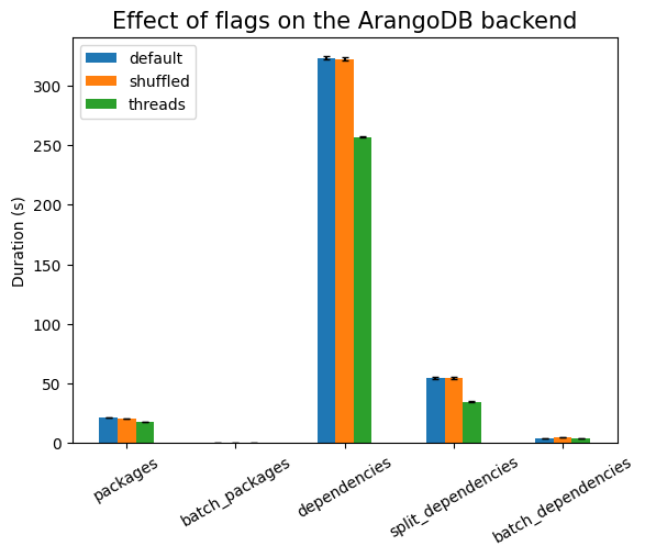
The pattern repeats if we zoom in to the fast ingestions.
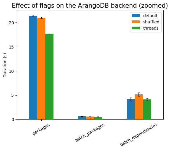
Next, we should look at how performance scales with the number of packages:
| Experiment | N | time (s) | stddev (s) |
|---|---|---|---|
packages |
10 | 0.024 | ±0.000 |
| 100 | 0.188 | ±0.002 | |
| 1000 | 1.763 | ±0.015 | |
| 10000 | 17.636 | ±0.053 | |
| 100000 | 178.450 | ±0.391 | |
| 1000000 | 1797.565 | ±1.371 | |
batch_packages |
10 | 0.003 | ±0.000 |
| 100 | 0.011 | ±0.000 | |
| 1000 | 0.059 | ±0.001 | |
| 10000 | 0.544 | ±0.017 | |
| 100000 | 6.316 | ±0.122 | |
dependencies |
10 | 0.244 | ±0.003 |
| 100 | 2.554 | ±0.017 | |
| 1000 | 25.688 | ±0.109 | |
| 10000 | 257.008 | ±0.571 | |
split_dependencies |
10 | 0.045 | ±0.008 |
| 100 | 0.361 | ±0.005 | |
| 1000 | 3.516 | ±0.035 | |
| 10000 | 34.910 | ±0.109 | |
| 100000 | 349.463 | ±0.540 | |
batch_dependencies |
10 | 0.008 | ±0.001 |
| 100 | 0.037 | ±0.001 | |
| 1000 | 0.346 | ±0.005 | |
| 10000 | 4.128 | ±0.230 | |
| 100000 | 50.329 | ±0.659 | |
bootstrap |
10 | 0.025 | ±0.040 |
| 100 | 0.024 | ±0.016 | |
| 1000 | 0.124 | ±0.020 | |
| 10000 | 0.860 | ±0.128 | |
| 100000 | 18.179 | ±6.233 | |
ecosystem |
10 | 0.021 | ±0.029 |
| 100 | 0.029 | ±0.003 | |
| 1000 | 0.281 | ±0.032 | |
| 10000 | 2.123 | ±0.081 | |
| 100000 | 35.537 | ±3.252 |
We can ingest 1 million packages directly. Unfortunately, batches of size 1 million result in OOM errors and we cannot otherwise ingest 1 million dependencies. In any case, ingestion is linear:
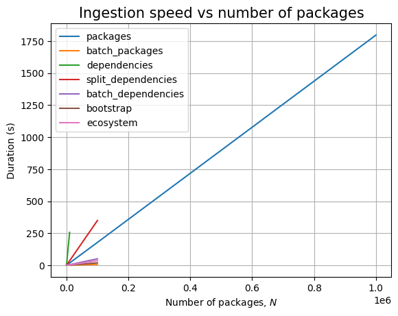
Since we cannot ingest 1 million packages and their dependencies, let’s zoom in:
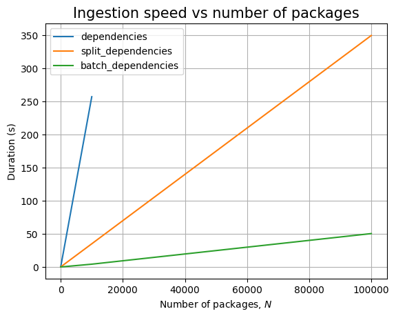
Querying, however, does not seem to be linear:
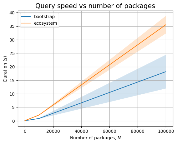
This is either because we have fewer than needed data points, or there is an actual accidental quadratic complexity in the way we wrote the retrieval. Further analysis is needed in a follow-up post.
For now, let’s look at the branching factor:
| Experiment | B | time (s) | stddev (s) |
|---|---|---|---|
packages |
2 | 18.249 | ±0.223 |
| 4 | 17.978 | ±0.205 | |
| 8 | 17.731 | ±0.096 | |
batch_packages |
2 | 0.589 | ±0.075 |
| 4 | 0.529 | ±0.011 | |
| 8 | 0.553 | ±0.010 | |
dependencies |
2 | 256.016 | ±0.650 |
| 4 | 256.839 | ±0.451 | |
| 8 | 257.093 | ±0.736 | |
split_dependencies |
2 | 35.074 | ±0.252 |
| 4 | 34.787 | ±0.069 | |
| 8 | 35.065 | ±0.124 | |
batch_dependencies |
2 | 4.132 | ±0.309 |
| 4 | 3.973 | ±0.054 | |
| 8 | 4.031 | ±0.041 | |
bootstrap |
2 | 1.193 | ±0.148 |
| 4 | 1.468 | ±0.162 | |
| 8 | 1.498 | ±0.317 | |
ecosystem |
2 | 2.685 | ±0.114 |
| 4 | 3.314 | ±0.134 | |
| 8 | 3.308 | ±0.289 |
Do we still have a decreasing time as \(B\) increases? Not really. Looking at packages, the time seems to be independent of \(B\):
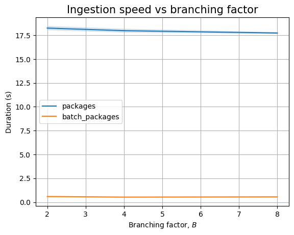
A similar trend shows up when looking at dependencies:
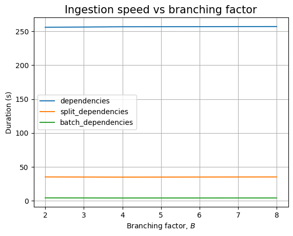
These can be explained by the fact that we just ingest in the proper
collection, with a given _key, without looking at what other connections
already exist. When we need to look at edges, we do see some impact, as
visible when we look at the queries:
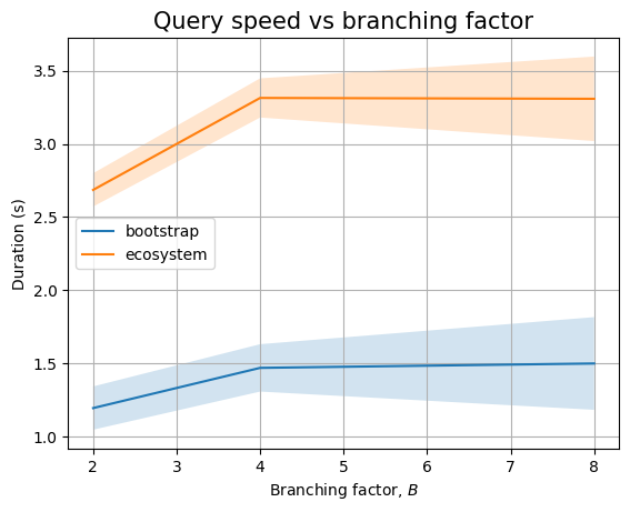
Here, in both cases we see an increase in run-time. However, this could also be considered to be constant time and affected by biased noise when \(B=2\). Further testing might be needed to determine an actual trend.
Meanwhile, let’s look at \(K\):
| Experiment | K | time (s) | stddev (s) |
|---|---|---|---|
dependencies |
1 | 52.232 | ±0.218 |
| 2 | 103.361 | ±0.375 | |
| 4 | 206.115 | ±1.132 | |
| 8 | 412.026 | ±1.636 | |
split_dependencies |
1 | 35.471 | ±0.107 |
| 2 | 35.335 | ±0.276 | |
| 4 | 34.922 | ±0.088 | |
| 8 | 34.269 | ±0.216 | |
batch_dependencies |
1 | 1.261 | ±0.141 |
| 2 | 1.889 | ±0.059 | |
| 4 | 3.454 | ±0.177 | |
| 8 | 6.803 | ±0.324 | |
bootstrap |
1 | 0.309 | ±0.065 |
| 2 | 0.453 | ±0.091 | |
| 4 | 0.906 | ±0.152 | |
| 8 | 2.255 | ±0.466 | |
ecosystem |
1 | 0.584 | ±0.038 |
| 2 | 1.001 | ±0.068 | |
| 4 | 2.208 | ±0.127 | |
| 8 | 5.151 | ±0.479 |
Here, the ingestion time is increasing linearly. There is a huge difference between ingesting dependencies one by one and ingesting them in batches or partial batches:
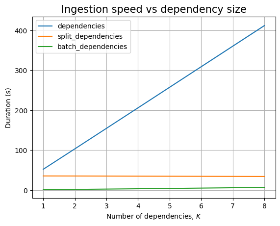
Querying also seems to be quadratic:
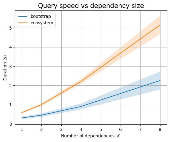
This gives more credence to the theory that there is an accidental quadratic complexity somewhere in the corresponding parts of the benchmarks. It is possible our query is not yet as performant as we’d need it to be (comparing to the equivalent Neo4j ones, these queries run slower).
A nice thing to note here before moving to the next database is that the measurements are less affected by noise. There are no more random stops due to GC runs.
Cayley 🔗
Cayley started as an unofficial Google product, but now is in its own GitHub organization. It has some really interesting differences compared with what we’ve seen so far.
Just like before, we use the database from within a docker container, which I start with:
docker run -p 64210:64210 --name cayley cayleygraph/cayley:latestThere is no access control, and I think this uses the default configuration. I’m seeing that the configuration allows me to change a storage backend, and I could choose between either several SQL databases or several noSQL ones. For now, let’s use the default, but keep in mind that performance might change if the backend changes.
There is no Python driver that we can use. But, we don’t need one. We only need to be able to send HTTP requests and use the short API (load it in the Swagger playground).
The UI allows me to insert or remove data, row by row. Data could also be ingested from a single file. The rest of the UI allows me to run queries and visualize the results, if the results are properly tagged. It is also possible to just see the graph traversal that the query would perform.
There doesn’t seem to be an easy way to drop the database, and there are no indexes to set up. The first part is troublesome, as it would basically mean that to delete old data I’d have to either traverse all nodes and delete them one by one, or stop the container (signals are not installed, so cleanup is not performed) and restart it. The latter cannot be done programmatically, so let’s do the former, at the risk of having the experiments need to run for longer.
Cayley is an RDF store: all graphs are stored as RDF triples. Well, actually, in Cayley we have quads instead of triples, mapping to the following Go struct:
type Quad struct {
 Subject   Value `json:“subject”`
 Predicate Value `json:“predicate”`
 Object    Value `json:“object”`
 Label     Value `json:“label,omitempty”`
}
This makes the graph be a Labeled Property Graph (LPG) instead of an RDF graph, something much closer to what Neo4j uses on the surface. But this is just semantics, the store is an RDF store with this additional attribute. We could use this label to define subgraphs or add additional named properties to a node, in case we have queries that need to operate on this subgraph (we won’t need it though, as can be seen in this section).
There are also multiple languages for querying: we can use GraphQL directly, we can use Gizmo (based on Gremlin/TinkerPop), or MQL, which, to the best of my understanding, was the initial query language. Since we’ll be testing another RDF-store database which also uses a Gremlin inspired language, let’s use Gizmo.
To test the backend, I’m sending simple HTTP requests using curl:
[...] λ curl -X POST -d "[{\"subject\":\"A\",\"predicate\":\"P0\",\"object\":\"B\"}]" -H 'Content-Type: application/json' http://localhost:64210/api/v2/write
{"result": "Successfully wrote 1 quads.", "count": 1}
[...] λ curl -X POST -d "[{\"subject\":\"A\",\"predicate\":\"P1\",\"object\":\"B\"}]" -H 'Content-Type: application/json' http://localhost:64210/api/v2/write
{"result": "Successfully wrote 1 quads.", "count": 1}
This should create 2 nodes (A and B) and 2 edges between them (P0 and
P1). However, when we retrieve this small graph we get a surprise:
[...] λ curl -X GET "http://localhost:64210/api/v2/query?lang=gizmo&qu=g.V().all()" | jq .
{
  "result": [
    {
      "id": "B"
    },
    {
      "id": "A"
    },
    {
      "id": "P0"
    },
    {
      "id": "P1"
    }
  ]
}
The edges are stored as vertices too, it seems. We can test that it is an actual edge:
[...] λ curl -X GET "http://localhost:64210/api/v2/query?lang=gizmo&qu=g.V(\"A\").out().all()" | jq .
{
  "result": [
    {
      "id": "B"
    },
    {
      "id": "B"
    }
  ]
}
We get two values of B because there are 2 edges coming out of A. We do
get just one node when asking for a certain path:
[...] λ curl -X GET "http://localhost:64210/api/v2/query?lang=gizmo&qu=g.V(\"A\").out(\"P0\").all()" | jq .
{
  "result": [
    {
      "id": "B"
    }
  ]
}
One more small detour to help in understanding this database before we start
the actual experiment: let’s estimate ingestion time and analyze how edges are
retrieved (without looking at the code :) ). I will ingest foo$${i} linked
by foobar to bar${i} for all values of i between 1 and 10 (or 100, or
1000), and foo0 linked to bar0 via edge. Then, I’ll time how long it
takes to find this special edge or the other ones:
[...] λ time (for i in `seq 1000`; do curl -X POST -d "[{\"subject\":\"foo${i}\",\"predicate\":\"foobar\",\"object\":\"bar${i}\"}]" -H 'Content-Type: application/json' http://localhost:64210/api/v2/write &> /dev/null; done);

real	1m49.216s
user	0m3.168s
sys	0m4.072s
[...] λ curl -X POST -d "[{\"subject\":\"foo0\",\"predicate\":\"edge\",\"object\":\"bar0\"}]" -H 'Content-Type: application/json' http://localhost:64210/api/v2/write
{"result": "Successfully wrote 1 quads.", "count": 1}
[...] λ time curl -X GET "http://localhost:64210/api/v2/query?lang=gizmo&qu=g.emit(g.V().out(\"edge\").count())"
{"result":[1]}

real	0m0.021s
user	0m0.006s
sys	0m0.003s
[...] λ time curl -X GET "http://localhost:64210/api/v2/query?lang=gizmo&qu=g.emit(g.V().out(\"foobar\").count())"
{"result":[1000]}

real	0m0.017s
user	0m0.004s
sys	0m0.004s
According to this minor experiment (not including full data here), ingesting is linear, while searching for an edge / node is seemingly constant time (at least for the small data under test). Based on this, we will define the following triple types (where we need to make sure that the nodes are unique across the entire instance, so we’d use a similar pURL encoding as in the ArangoDB case):
ecosystem - has_namespace - namespacenamespace - has_name - namename - has_version - versionversion - has_dependency - dependencydependency - has_target - version
We could have defined all edges (or at least those in the package trie) to be
has, which might make some queries faster and other slower. If someone with
more experience in Cayley has a better suggestion I’ll definitely update and
run the experiments again (in another post).
I haven’t found a reason to use the 4th element in the quad. But, just like above, if anyone with more Cayley experience has a suggestion that could improve performance I will test that one too.
Before moving on, there is just one more observation to make: since edges are also nodes and deleting a node also deletes everything that is connected to it, we can delete everything in the database by deleting edges (5 statements in total, regardless of \(N\) – but still requiring traversing the entire database) instead of deleting nodes:
[...] λ curl -X POST -d "\"foobar\"" -H 'Content-Type: application/json' http://localhost:64210/api/v2/node/delete
{"result": "Successfully deleted 1 nodes.", "count": 1}
With this being said, here is the code to set-up and tear-down the database:
class Cayley(Experiment):
    def __init__(self, N: int, B: int, K: int, shuffle: bool = True, threaded: bool = True):
        super().__init__(N, B, K, shuffle, threaded)
        host = 'http://localhost:64210'
        self.write_url = f'{host}/api/v2/write'
        self.delete_url = f'{host}/api/v2/node/delete'
        self.query_url = f'{host}/api/v2/query?lang=gizmo&qu='

    def _do_clean(self):
        edges = ['has_namespace', 'has_name', 'has_version',
                 'has_dependency', 'has_target']

        with requests.Session() as s:
            for edge in edges:
                s.post(self.delete_url, json=edge)

    # ...
We just store the 3 URLs involved in the REST API and delete the data on
clean by sending the corresponding POST request. There is no need for
__del__ or setup.
Ingesting packages is trivial once we extract a helper to build the JSON part of the request:
class Cayley(Experiment):
    # ...

    def _make_package_object(self, package: Package):
        ecosystem = f'e_{package.ecosystem}'
        namespace = f'{package.ecosystem}_{package.namespace}'
        name = f'{namespace}_{package.name}'
        return [
            { 'subject': ecosystem, 'predicate': 'has_namespace', 'object': namespace },
            { 'subject': namespace, 'predicate': 'has_name', 'object': name },
            { 'subject': name, 'predicate': 'has_version', 'object': package.version },
        ]

    def _do_ingest_package(self, package: Package):
        data = self._make_package_object(package)
        with requests.Session() as s:
            s.post(self.write_url, json=data)

    def _do_ingest_batch_packages(self, packages: Sequence[Package]):
        data = []
        for p in packages:
            data.extend(self._make_package_object(p))
        with requests.Session() as s:
            s.post(self.write_url, json=data)

    # ...
The only difference for batch ingestion is just the fact that we’re sending a larger JSON.
A similar pattern occurs when ingesting dependencies:
class Cayley(Experiment):
    # ...

    def _make_dependency_object(self, dependency: Dependency):
        parent = dependency.parent.version
        target = dependency.target.version
        dependency_label = f'{parent}-{target}'
        return [
            { 'subject': parent, 'predicate': 'has_dependency', 'object': dependency_label },
            { 'subject': dependency_label, 'predicate': 'has_target', 'object': target },
        ]

    def _do_ingest_dependency(self, dependency: Dependency):
        data = self._make_dependency_object(dependency)
        with requests.Session() as s:
            s.post(self.write_url, json=data)

    def _do_ingest_batch_dependencies(self, dependencies: Sequence[Dependency]):
        data = []
        for d in dependencies:
            data.extend(self._make_dependency_object(d))
        with requests.Session() as s:
            s.post(self.write_url, json=data)

    # ...
The interesting parts arise on queries. The intuition is that each query should be viewed as a collection of path traversals, and each new query component applies to the current node only. Thus, we have to construct paths between nodes involved in (in)equalities. In order to have a reference to a node, we have to bind it via a function argument. So:
class Cayley(Experiment):
    # ...

    def _do_query_bootstrap(self):
        query = """
name_nodes = g.V().has("has_version").unique()

path_to_target = g.M().out("has_dependency").out("has_target")

name_nodes.ForEach(function(n) {
  g.V(n.id)
   .out("has_version").tag("parent")
   .follow(path_to_target).tag("target")
   .in("has_version")
   .is(n.id)
   .all()
})
"""
        with requests.Session() as s:
            response = s.get(f'{self.query_url}{query}')
        result = response.json()['result'] or []
        return [(r['parent'], r['target']) for r in result]

    # ...
We select all the name nodes in name_nodes, making sure they only show up a
single time. Then, for each of these nodes, we start a traversal to find the
parent package, the target package, and the name node corresponding to this
target package. If the name is the same as the node we started with, then we
have a bootstrap dependency.
For cross-ecosystem queries, we need to use except to eliminate paths. The
intuition is that except will not output the current path if the current
node (where except is called on) is also the final node of the traversal
given as argument:
class Cayley(Experiment):
    # ...

    def _do_query_ecosystem(self):
        query = """
ecosystems = g.V().has("has_namespace").unique()

to_version = g.M().out("has_namespace").out("has_name").out("has_version")
to_target = g.M().out("has_dependency").out("has_target")

ecosystems.ForEach(function(e1) {
  g.V(e1.id)
   .follow(to_version).tag("parent")
   .follow(to_target).tag("target")
   .followR(to_version)
   .except(g.V(e1.id))
   .all()
})
"""
        with requests.Session() as s:
            response = s.get(f'{self.query_url}{query}')
        result = response.json()['result'] or []
        return [(r['parent'], r['target']) for r in result]
With this, we can now run the experiments. Just like in the ArangoDB case, we don’t have indexes (but this time because they are not exposed to the interface, the Cayley backend will create them according to the storage backend being used).
First, let’s look at the effect of flags:
| Experiment | type | time (s) | stddev (s) |
|---|---|---|---|
packages |
1106.758 | ±33.797 | |
| shuffled | 1574.324 | ±7.767 | |
| threads | 1473.034 | ±15.679 | |
batch_packages |
2.268 | ±0.381 | |
| shuffled | 3.855 | ±0.085 | |
| threads | 4.863 | ±0.090 | |
batch_dependencies |
12.649 | ±1.344 | |
| shuffled | 23.787 | ±1.020 | |
| threads | 18.231 | ±0.508 |
Cayley is slow, so we cannot ingest 10k dependencies except in a whole batch. Overall, it seems that adding threads makes things slower:
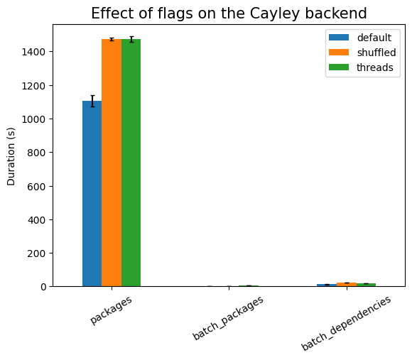
Same pattern occurs if we zoom in to the batch ingestions:
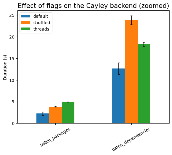
As such, in the rest of the experiments, we won’t use threads.
Looking at performance as \(N\) increases, we see a very bleak figure:
| Experiment | N | time (s) | stddev (s) |
|---|---|---|---|
packages |
10 | 1.011 | ±0.043 |
| 100 | 13.529 | ±0.810 | |
| 1000 | 139.583 | ±4.901 | |
| 10000 | 1106.758 | ±33.797 | |
batch_packages |
10 | 0.163 | ±0.025 |
| 100 | 0.312 | ±0.033 | |
| 1000 | 0.587 | ±0.045 | |
| 10000 | 2.268 | ±0.381 | |
| 100000 | 34.408 | ±2.269 | |
| 1000000 | 765.545 | ±120.006 | |
dependencies |
10 | 12.985 | ±0.631 |
| 100 | 192.475 | ±7.934 | |
| 1000 | 1894.200 | ±20.997 | |
split_dependencies |
10 | 2.469 | ±0.077 |
| 100 | 28.534 | ±0.741 | |
| 1000 | 346.011 | ±3.861 | |
batch_dependencies |
10 | 0.437 | ±0.027 |
| 100 | 0.640 | ±0.063 | |
| 1000 | 1.681 | ±0.092 | |
| 10000 | 12.649 | ±1.344 | |
| 100000 | 481.862 | ±0.250 | |
bootstrap |
10 | 2.819 | ±0.035 |
| 100 | 2.857 | ±0.043 | |
| 1000 | 0.261 | ±0.010 | |
| 10000 | 2.555 | ±0.041 | |
| 100000 | 24.906 | ±0.272 | |
ecosystem |
10 | 0.011 | ±0.000 |
| 100 | 0.049 | ±0.001 | |
| 1000 | 0.085 | ±0.002 | |
| 10000 | 0.360 | ±0.007 | |
| 100000 | 3.051 | ±0.013 |
We can ingest batch packages up to 1 million in a time that is faster than ArangoDB used:
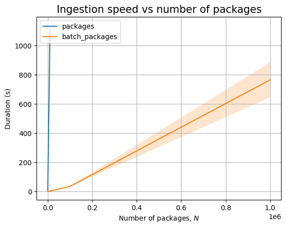
However, this is the only win. Dependencies take longer to ingest, and only batches can ingest high enough number of packages and their dependencies:
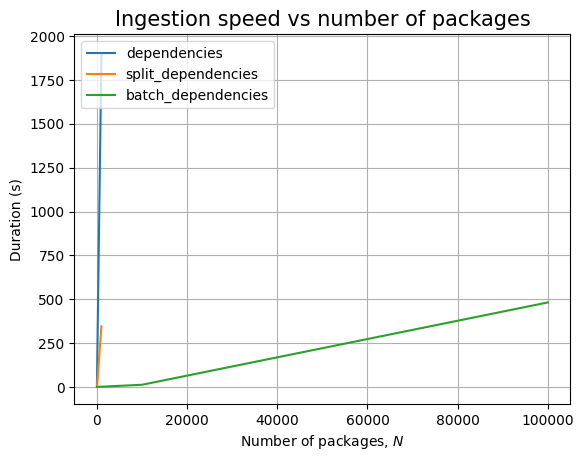
Query time increases linearly:
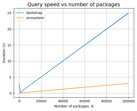
However, note how bootstrap queries are now slower than ecosystem ones! This is a complete reversal from previous instances.
A similar picture can be drawn when looking at the branching factor:
| Experiment | B | time (s) | stddev (s) |
|---|---|---|---|
packages |
2 | 908.986 | ±85.983 |
| 4 | 1155.119 | ±64.424 | |
| 8 | 1090.643 | ±92.321 | |
batch_packages |
2 | 0.785 | ±0.064 |
| 4 | 0.875 | ±0.027 | |
| 8 | 0.940 | ±0.030 | |
batch_dependencies |
2 | 8.595 | ±1.335 |
| 4 | 9.584 | ±0.126 | |
| 8 | 9.859 | ±0.163 | |
bootstrap |
2 | 3.500 | ±0.032 |
| 4 | 5.589 | ±0.058 | |
| 8 | 5.885 | ±0.042 | |
ecosystem |
2 | 3.171 | ±0.011 |
| 4 | 3.454 | ±0.038 | |
| 8 | 3.754 | ±0.017 |
Package ingestion time increases linearly with \(B\):
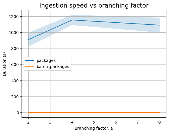
A similar pattern occurs for dependencies (modulo large noise):
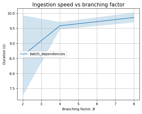
And it is very possible that we see a similar pattern when looking at the queries:
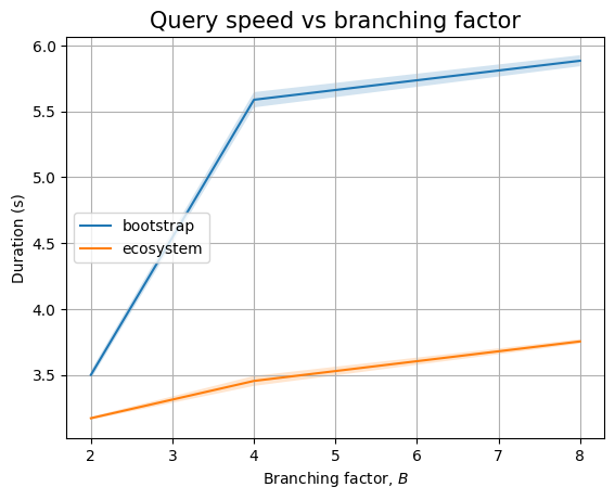
Here, again, it takes longer to run a bootstrap query than an ecosystem one.
Finally, similar patterns are visible when looking at the impact of \(K\):
| Experiment | K | time (s) | stddev (s) |
|---|---|---|---|
batch_dependencies |
1 | 3.906 | ±0.131 |
| 2 | 5.192 | ±0.279 | |
| 4 | 8.158 | ±0.326 | |
| 8 | 18.304 | ±1.445 | |
bootstrap |
1 | 3.890 | ±0.046 |
| 2 | 4.280 | ±0.019 | |
| 4 | 5.470 | ±0.060 | |
| 8 | 10.891 | ±0.106 | |
ecosystem |
1 | 3.759 | ±0.017 |
| 2 | 3.879 | ±0.023 | |
| 4 | 5.178 | ±0.035 | |
| 8 | 5.856 | ±0.061 |
In this case, we can put all 3 lines on the same graph:
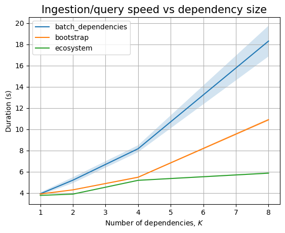
It is very possible that changing the backend Cayley uses might result in some performance gains, but the default one does not seem to perform adequately. Similarly, perhaps some slowdown can be optimized away if we are not required to send REST requests and instead communicate directly with the backend.
TerminusDB 🔗
TerminusDB is at the confluence of databases we’ve seen so far. It is a document store, like ArangoDB. It uses a semantic web ontology, like Cayley, with a powerful query language, and with all data normalized to RDF triples. It is a graph database like Neo4j, but with a clever representation of the graph as a document. Thus, we can see it as a knowledge graph database. These design choices mean that the database has to be schema-first: we have to define a schema for all data and this schema will be validated on each mutation.
Given the storage as RDF, we have indexes built for us
already (so the -i option is useless) and we need
to perform extra steps if we want to have duplicate relations (which we
don’t). Unfortunately, the Python client seems to have issues with
multi-threading, so we won’t be able to test the effect of -t either.
To increase performance, given the fact that RDF triples have common prefixes, TerminusDB uses succinct data structures and delta encoding of changes. This additionally enables support for MVCC and gigantic graphs.
TerminusDB developers already wrote a blog post about a usecase similar to what we want in GUAC.
Unlike the databases we’ve seen so far, TerminusDB offers a full script to manage the entire set of docker based workflows. It is just a wrapper around setting the needed environment variables and getting the proper image, so there’s nothing that cannot be run as a command directly.
To use it, we need to clone a separate repository before running the script:
[...]$ git clone https://github.com/terminusdb/terminusdb-bootstrap
[...]$ cd terminusdb-bootstrap
[...]$ # prepare environment variables ...
[...]$ ./terminusdb-container run
Subsequent runs need to first stop container and remove data:
[...]$ ./terminusdb-container stop
[...]$ ./terminusdb-container rm
[...]$ ./terminusdb-container run
Since I’m using NixOS, the above has to be run in a proper environment (and
change the shebang line to the real path to bash):
nix-shell -p python311Regarding clients, we might not need them, given that TerminusDB now comes with a GraphQL client that automatically generates GraphQL schema based on schema definition. However, in order to not compare apples with oranges, I’ll use the Python client. The wheel is not available on NixOS packages search index, so we’ll need to create a custom Nix shell to import it (this could be improved, but after I learn more Nix):
{ pkgs ? import <nixpkgs> {} }:

let
  local_com2ann = ps: with ps; [
    (
      buildPythonPackage rec {
        pname = "com2ann";
        version = "0.3.0";
        src = fetchPypi {
          inherit pname version;
          sha256 = "sha256-DaXjkAKSBX5cSl4zsh/kiBe0kjQ3oJXmpnff+Us9ThA=";
        };
        doCheck = false;
      }
    )
  ];
  local_shed = ps: with ps; [
    (
      buildPythonPackage rec {
        pname = "shed";
        version = "2023.5.1";
        src = fetchPypi {
          inherit pname version;
          sha256 = "sha256-jbpQsbMEBpMKKRtgp1p3R0b5rQzJAl2ZHpfYOhEKi/k=";
        };
        doCheck = false;
        buildInputs = [
          autoflake
          black
          isort
          libcst
          pyupgrade
          (pkgs.python311.withPackages local_com2ann)
        ];
      }
    )
  ];
  local_terminus = ps: with ps; [
    (
      buildPythonPackage rec {
        pname = "terminusdb-client";
        version = "10.2.3";
        src = fetchPypi {
          inherit pname version;
          sha256 = "sha256-QzifsW4I76B5hK1pmlyclQeRHjyjRPw/DBLM57BlmLs=";
        };
        doCheck = false;
        buildInputs = [
          autoflake
          black
          click
          isort
          libcst
          pyupgrade
          tqdm
          (pkgs.python311.withPackages local_com2ann)
          (pkgs.python311.withPackages local_shed)
        ];
        propagatedBuildInputs = [
          numpydoc
          requests
          typeguard
        ];
      }
    )
  ];
in
  with pkgs;
  mkShell {
    nativeBuildInputs = [
      (python311.withPackages local_terminus)
    ];

    shellHook = ''
      export PS1="[\[\033[01;32m\]nix-shell\[\033[00m\]:\W] \[\033[01;32m\]λ\[\033[00m\] "
    '';
  }
Now, we can begin setting up and database for the tests as well as writing the code for tearing down the tests.
class Terminus(Experiment):
    def __init__(self, N: int, B: int, K: int, shuffle: bool = True, threaded: bool = True):
        super().__init__(N, B, K, shuffle, threaded)
        import terminusdb_client as terminus
        self._client = terminus.Client("http://localhost:6363/")
        self._client.connect()

    def __del__(self):
        self._client.close()

    def setup(self, indexes: bool = True):
        self._db = "test"
        if not self._client.get_databases():
            self._client.create_database(self._db)
        self._client.connect(db=self._db)
        schemas = self._client.get_all_documents(graph_type='schema', as_list=True)
        if len(schemas) < 2:
            schema = [
                { '@type': 'Class', '@id': 'Ecosystem' },
                { '@type': 'Class', '@id': 'Namespace', 'ecosystem': 'Ecosystem' },
                { '@type': 'Class', '@id': 'Name', 'namespace': 'Namespace' },
                { '@type': 'Class', '@id': 'Version', 'name': 'Name' },
                { '@type': 'Class', '@id': 'Dependency',
                  'parent': 'Version', 'target': 'Version' },
            ]
            self._client.insert_document(schema, graph_type='schema')

    def _do_clean(self):
        self._client.delete_database(self._db, 'admin', force=True)

    # ...
Because TerminusDB enforces schema for all documents, we have to declare it,
but only once. There is a default schema already present, so we check that the
number of schemas is at least 2 when we want to skip declaring our custom
schema. The test specific schema is created by ingesting a document for the
schema meta-graph. In our chosen schema, we have included links from
children nodes to their parents in the package tries, instead of going the
reverse way:
            schema = [
                { '@type': 'Class', '@id': 'Ecosystem',
                  'namespace': { '@type': 'Set', '@class': 'Namespace' }},
                { '@type': 'Class', '@id': 'Namespace',
                  'name': { '@type': 'Set', '@class': 'Name' }},
                { '@type': 'Class', '@id': 'Name',
                  'version': { '@type': 'Set', '@class': 'Version' }},
                { '@type': 'Class', '@id': 'Version',
                  'dependency': { '@type': 'Set', '@class': 'Dependency' }},
                { '@type': 'Class', '@id': 'Dependency', 'target': 'Version' },
            ]
Going from parent node to set of children nodes means that each time we do an ingestion we have to modify both the parent node and the child node, even in the cases where the parent was already ingested from a previous mutation. Hence, we prefer to use the reverse relationship, as that should increase performance.
This time, instead of writing the queries directly, let’s use the Python client’s API (in fact, documentation does not seem to point to the possibility of writing queries directly). We will use a helper function to create the JSON documents that the API expects:
class Terminus(Experiment):
    # ...

    def _make_package_docs(self, package: Package):
        ecosystem = f'Ecosystem/{package.ecosystem}'
        namespace = f'Namespace/{package.ecosystem}_{package.namespace}'
        name = f'Name/{package.ecosystem}_{package.namespace}_{package.name}'
        version = f'Version/{package.version}'
        return [
            { '@type': 'Ecosystem', '@id': ecosystem },
            { '@type': 'Namespace', '@id': namespace, 'ecosystem': ecosystem },
            { '@type': 'Name', '@id': name, 'namespace': namespace },
            { '@type': 'Version', '@id': version, 'name': name },
        ]

    def _do_ingest_package(self, package: Package):
        self._client.update_document(self._make_package_docs(package))

    def _do_ingest_batch_packages(self, packages: Sequence[Package]):
        def _update(d, kv):
            if kv['@id'] not in d: d[kv['@id']] = kv

        ecosystems = {}
        namespaces = {}
        names = {}
        versions = {}
        for p in packages:
            ecosystem, namespace, name, version = self._make_package_docs(p)
            _update(ecosystems, ecosystem)
            _update(namespaces, namespace)
            _update(names, name)
            _update(versions, version)
        docs = []
        for ecosystem in ecosystems: docs.append(ecosystems[ecosystem])
        for namespace in namespaces: docs.append(namespaces[namespace])
        for name in names: docs.append(names[name])
        for version in versions: docs.append(versions[version])
        self._client.update_document(docs)

    # ...
We have some constraints that we need to take care of. First, because of the schema validation, our IDs are required to follow a specific pattern (class name followed by desired identifier). Next, TerminusDB doesn’t allow us to change the same document twice in the API call, so when doing batch ingestion we actually have to first deduplicate each node. This will result in some slowdown, as we will see later.
Ingesting dependencies follows a similar pattern:
class Terminus(Experiment):
    # ...

    def _make_dependency_doc(self, dependency: Dependency):
        parent = dependency.parent.version
        target = dependency.target.version
        label = f'Dependency/{parent}-{target}'
        parent = f'Version/{parent}'
        target = f'Version/{target}'
        return { '@type': 'Dependency', '@id':label,
                 'parent': parent, 'target': target }

    def _do_ingest_dependency(self, dependency: Dependency):
        self._client.update_document([self._make_dependency_doc(dependency)])

    def _do_ingest_batch_dependencies(self, dependencies: Sequence[Dependency]):
        deps = {}
        for d in dependencies:
            dd = self._make_dependency_doc(d)
            if dd['@id'] not in deps: deps[dd['@id']] = dd
        docs = [deps[k] for k in deps]
        self._client.update_document(docs)

    # ...
For read queries, we will use the WOQLQuery API,
together with a helper to parse the response and eliminate the class prefixes:
class Terminus(Experiment):
    # ...

    def _process_response(self, response):
        def parse_version_from_IRI(iri):
            return iri[8:]

        if response['api:status'] != 'api:success':
            print(response)
            return []
        ret = []
        for binding in response['bindings']:
            parent = parse_version_from_IRI(binding['Parent'])
            target = parse_version_from_IRI(binding['Target'])
            ret.append((parent, target))
        return ret

    def _do_query_bootstrap(self):
        from terminusdb_client import WOQLQuery
        query = WOQLQuery().select('v:Parent', 'v:Target').woql_and(
                WOQLQuery().triple('v:Dep', 'rdf:type', '@schema:Dependency'),
                WOQLQuery().triple('v:Dep', '@schema:parent', 'v:Parent'),
                WOQLQuery().triple('v:Parent', '@schema:name', 'v:Name'),
                WOQLQuery().triple('v:Dep', '@schema:target', 'v:Target'),
                WOQLQuery().triple('v:Target', '@schema:name', 'v:Name'))
        return self._process_response(self._client.query(query))

    def _do_query_ecosystem(self):
        from terminusdb_client import WOQLQuery
        query = WOQLQuery().select('v:Parent', 'v:Target').woql_and(
                WOQLQuery().triple('v:Dep', 'rdf:type', '@schema:Dependency'),
                WOQLQuery().triple('v:Dep', '@schema:parent', 'v:Parent'),
                WOQLQuery().triple('v:Parent', '@schema:name', 'v:NameP'),
                WOQLQuery().triple('v:NameP', '@schema:namespace', 'v:NSP'),
                WOQLQuery().triple('v:NSP', '@schema:ecosystem', 'v:EcosystemP'),
                WOQLQuery().triple('v:Dep', '@schema:target', 'v:Target'),
                WOQLQuery().triple('v:Target', '@schema:name', 'v:NameT'),
                WOQLQuery().triple('v:NameT', '@schema:namespace', 'v:NST'),
                WOQLQuery().triple('v:NST', '@schema:ecosystem', 'v:EcosystemT'),
                WOQLQuery().woql_not(WOQLQuery().eq('v:EcosystemP', 'v:EcosystemT')))
        return self._process_response(self._client.query(query))
Looking at the timing of the experiments, we can see that the performance here is again not great. In fact, we can only run batch ingestion for 10k packages, so this is worse than Cayley.
| Experiment | type | time (s) | stddev (s) |
|---|---|---|---|
batch_packages |
2.933 | ±0.119 | |
| shuffled | 2.904 | ±0.026 | |
batch_dependencies |
21.954 | ±0.062 | |
| shuffled | 22.326 | ±0.100 |
As expected, there is not much difference between passing the data in order or shuffling it. We can see the same on the graph:
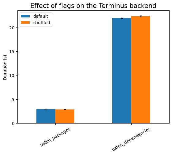
More interesting is the scaling with regards to \(N\):
| Experiment | N | time (s) | stddev (s) |
|---|---|---|---|
packages |
10 | 1.512 | ±0.053 |
| 100 | 16.173 | ±0.211 | |
| 1000 | 248.307 | ±2.966 | |
batch_packages |
10 | 0.156 | ±0.016 |
| 100 | 0.223 | ±0.013 | |
| 1000 | 0.454 | ±0.006 | |
| 10000 | 2.904 | ±0.026 | |
| 100000 | 26.739 | ±0.098 | |
| 1000000 | 275.210 | ±7.791 | |
dependencies |
10 | 10.477 | ±0.287 |
| 100 | 173.126 | ±0.475 | |
split_dependencies |
10 | 2.614 | ±0.237 |
| 100 | 29.931 | ±0.364 | |
| 1000 | 725.362 | ±1.054 | |
batch_dependencies |
10 | 0.322 | ±0.027 |
| 100 | 0.576 | ±0.046 | |
| 1000 | 2.591 | ±0.048 | |
| 10000 | 21.954 | ±0.062 | |
| 100000 | 221.753 | ±1.604 | |
bootstrap |
10 | 0.054 | ±0.063 |
| 100 | 0.033 | ±0.001 | |
| 1000 | 0.191 | ±0.001 | |
| 10000 | 1.891 | ±0.020 | |
| 100000 | 20.172 | ±0.125 | |
ecosystem |
10 | 0.032 | ±0.022 |
| 100 | 0.061 | ±0.005 | |
| 1000 | 0.437 | ±0.006 | |
| 10000 | 4.475 | ±0.024 | |
| 100000 | 46.833 | ±0.097 |
We have a clear imbalance: we can ingest up to 1 million packages in a batch, but anything not using batches can only be ingested up to \(N = 1000\). As such, we will zoom in on the graph from the start:
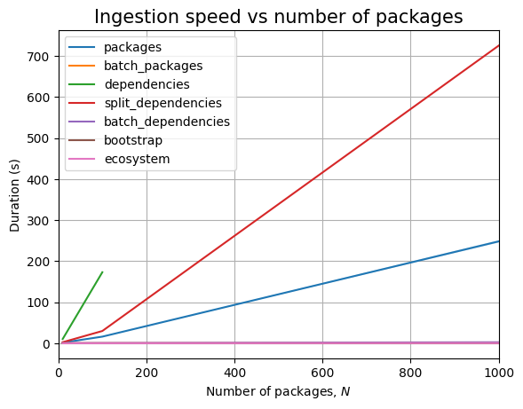
If we look at queries only, we have the following graph:
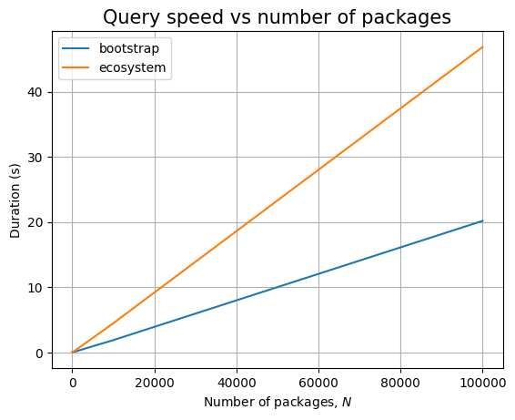
We are back to the general case we have seen so far (excluding Cayley): the query for bootstrap packages is faster than the query for cross-ecosystem dependencies.
Looking at \(B\), we again expect a very small effect:
| Experiment | B | time (s) | stddev (s) |
|---|---|---|---|
batch_packages |
2 | 2.818 | ±0.025 |
| 4 | 2.888 | ±0.017 | |
| 8 | 3.058 | ±0.021 | |
batch_dependencies |
2 | 21.806 | ±0.113 |
| 4 | 21.904 | ±0.158 | |
| 8 | 22.060 | ±0.212 | |
bootstrap |
2 | 2.070 | ±0.019 |
| 4 | 1.903 | ±0.017 | |
| 8 | 1.906 | ±0.017 | |
ecosystem |
2 | 4.150 | ±0.021 |
| 4 | 4.463 | ±0.027 | |
| 8 | 4.620 | ±0.044 |
And indeed, the data shows near constant time:
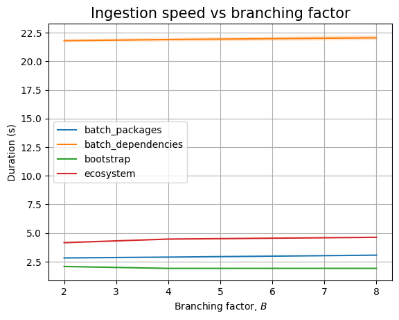
But, actually, if we zoom in to the queries, we see a similar pattern as in the Neo4j case: ecosystem queries get more expensive while bootstrap ones seem to be at most constant, if not decreasing:
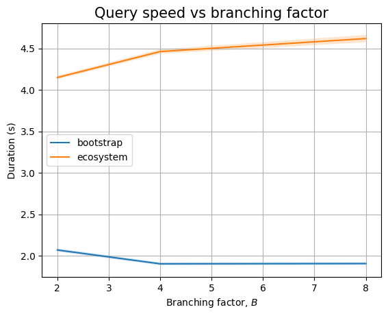
This matches the intuition on number of graph nodes that need to be looked at during query execution.
Now, let’s move forward and look at the effect of \(K\):
| Experiment | K | time (s) | stddev (s) |
|---|---|---|---|
batch_dependencies |
1 | 7.075 | ±0.070 |
| 2 | 10.803 | ±0.054 | |
| 4 | 18.324 | ±0.085 | |
| 8 | 33.486 | ±0.228 | |
bootstrap |
1 | 0.398 | ±0.004 |
| 2 | 0.760 | ±0.010 | |
| 4 | 1.522 | ±0.016 | |
| 8 | 3.065 | ±0.011 | |
ecosystem |
1 | 0.931 | ±0.010 |
| 2 | 1.805 | ±0.015 | |
| 4 | 3.639 | ±0.045 | |
| 8 | 7.219 | ±0.031 |
Here, everything seems to increase linearly. Plotting reveals that this is indeed the pattern:
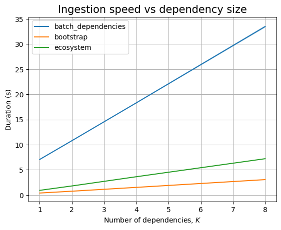
In summary, TerminusDB seems to have similar performance patterns as Neo4j and Arango, but is much more expensive: when looking at fixed \(N,B,K\) values, the ingestion/querying runs much much slower.
Time to move to the next database.
JanusGraph 🔗
JanusGraph database might look very similar to Cayley: it is also a triple store (more so than Cayley was) and it also relies on TinkerPop/Gremlin as the query language. This makes it easier to add node properties, though; we no longer need to ingest triples as JSON documents! Just like Cayley, there are multiple storage backends. As such, this section should be mostly self-explanatory.
As usual, we start a docker container first:
sudo docker run -p 8182:8182 --name janusgraph janusgraph/janusgraphAnd we start a Nix shell with all the needed dependencies using
nix-shell -p python311Packages.gremlinpythonNote that we are using the official Gremlin package, not one for JanusGraph. The reference manual looks well documented, with additional stories. However, the documentation assumes Java usage, with very few examples in other languages. In fact, there is even lack of support for some aspects.
For example, the JanusGraph implementation does not support the new merge operations. So, as we will see soon, we need to write a more complex query to only insert a vertex if not already present. For another example, the Python driver receives both Python errors and Java errors from the backend, as well as errors caused by not yet implemented conversions, etc. There is no clear formatting between the two, and reading an error message you have to imagine where it could come from and what the reason could be. The code for the Python driver is almost not documented, hence most of the time I was preparing for this section has been spent in trying to solve driver returned error. For a final example, the Python driver does not support setting indexes. Even if the database logs are suggesting that we add indexes, we cannot do this from Python. Thus, we will consider that this is not possible (as we want to do it programmatically, instead of doing this out-of-band, when the database is set up).
Threading support seems incomplete. Although I have not encountered deadlocks (like in the case of TerminusDB), I have seen multiple times errors due to locking timeouts. Hence, we will assume threading should not be tested.
The setup and tear down code is mostly trivial:
class JanusGraph(Experiment):
    def __init__(self, N: int, B: int, K: int, shuffle: bool = True, threaded: bool = True):
        super().__init__(N, B, K, shuffle, threaded)
        from gremlin_python.driver.driver_remote_connection import DriverRemoteConnection
        from gremlin_python.process.anonymous_traversal import traversal
        from gremlin_python.process.graph_traversal import __, label, outV
        from gremlin_python.process.traversal import P
        self._client = DriverRemoteConnection('ws://localhost:8182/gremlin', 'g')
        self._g = traversal().withRemote(self._client)
        self.__P = P
        self.__U = __.unfold
        self.__V = __.addV
        self.__E = __.addE
        self.__O = outV
        self.__I = __.in_
        self.__IE = __.inE

    def __del__(self):
        self._client.close()

    def setup(self, indexes: bool = True):
        pass

    def _do_clean(self):
        self._g.E().drop().iterate()
        self._g.V().drop().iterate()

    # ...
We need to import multiple paths and instead of spending the cost of import in the ingestion callbacks we save the needed functions in class variables. We could have used global imports but then we need to make sure only the imports needed for the current experiment are active (either by commenting the others or separating each class into its own file and importing based on experiment kind).
Moving on, let’s insert packages:
class JanusGraph(Experiment):
    # ...

    def _find_or_add_node(self, label):
        return self._g.V().hasLabel(label).fold().coalesce(
                self.__U(), self.__V(label)).toList()[0].id

    def _ensure_edge(self, parent, label, target):
        self._g.V(parent).as_('parent').V(target).as_('target').coalesce(
                self.__IE(label).where(self.__O().as_('parent')),
                self.__E(label).from_('parent').to('target')).iterate()

    def _do_ingest_package(self, package: Package):
        ecosystem = f'e_{package.ecosystem}'
        namespace = f'{package.ecosystem}_{package.namespace}'
        name = f'{namespace}_{package.name}'
        version = package.version

        ecosystem = self._find_or_add_node(ecosystem)
        namespace = self._find_or_add_node(namespace)
        name = self._find_or_add_node(name)
        version = self._find_or_add_node(version)

        self._ensure_edge(ecosystem, 'has_namespace', namespace)
        self._ensure_edge(namespace, 'has_name', name)
        self._ensure_edge(name, 'has_version', version)

    def _do_ingest_batch_packages(self, packages: Sequence[Package]):
        for package in packages:
            self._do_ingest_package(package)

    # ...
Going from the bottom-up: since I could not find a way to ingest a full list of packages at once and the ingestion of a single package is complex (as we will see shortly), the only way to do batch ingestion is to manually write the loop. This means we won’t expect significant differences between batched and non-batched ingestion.
Next, to ingest packages, we need to add vertices and edges between them, making sure to not add duplicates. Focusing on a vertex for now, we could have run 2 queries, like in
(list(self._g.V().hasLabel(label)) or list(self._g.addV(label)))[0]But each query needs to be serialized and sent to the JVM running the database. So, we should try to do a single query. On the other extreme, we could ingest all 4 vertexes at once:
        self._g.V().hasLabel(ecosystem).fold() .\
                coalesce(self.__U(), self.__V(ecosystem)) .\
                V().hasLabel(namespace).fold(). \
                coalesce(self.__U(), self.__V(namespace)) .\
                V().hasLabel(name).fold(). \
                coalesce(self.__U(), self.__V(name)) .\
                V().hasLabel(version).fold(). \
                coalesce(self.__U(), self.__V(version)) .\
                iterate()
The downside of this is that we cannot then bind to the nodes to add the edges. So we’d need separate queries to locate these vertexes, using their labels (which turns out to be slower than the chosen approach).
Hence, we will use the fold-coalesce-unfold approach:
        return self._g.V().hasLabel(label).fold().coalesce(
                self.__U(), self.__V(label)).toList()[0].id
Here, fold forces traversal to collect all results so far into a single
list. In our case, we will have a list of either one node or 0. Then
coalesce can be viewed as a select statement, the first argument is an
expression that could evaluate to some results (in general, this would be
extracting the elements from the folded list, one by one, if present). If no
results are available from first expression, then the second argument of
coalesce gets executed and this is where we insert the node.
For the edge ingestion, we first locate the 2 endpoints using their IDs (so
this should be fast) and then use coalesce to identify if there is an
edge linking them or not. If there is no edge, we create it.
Ingesting dependencies uses the same helpers:
class JanusGraph(Experiment):
    # ...

    def _do_ingest_dependency(self, dependency: Dependency):
        parent = dependency.parent.version
        target = dependency.target.version
        dependency = f'dep_{parent}-{target}'

        dependency = self._find_or_add_node(dependency)
        parent = self._find_or_add_node(parent)
        target = self._find_or_add_node(target)

        self._ensure_edge(parent, 'has_dependency', dependency)
        self._ensure_edge(dependency, 'has_target', target)

    def _do_ingest_batch_dependencies(self, dependencies: Sequence[Dependency]):
        for dependency in dependencies:
            self._do_ingest_dependency(dependency)

    # ...
Querying is mostly similar as in the Cayley case. Except we cannot save
traversals to variables, so everything has to be written in a single
expression. We also don’t have ForEach, we have to use where instead.
class JanusGraph(Experiment):
    # ...

    def _do_query_bootstrap(self):
        result = self._g.V().as_('v1').\
                out('has_version').as_('parent').\
                out('has_dependency').out('has_target').as_('target').\
                where(self.__I('has_version').as_('v1')).\
                select('v1','parent','target').\
                toList()
        return [(r['parent'].label, r['target'].label) for r in result]

    def _do_query_ecosystem(self):
        result = self._g.V().as_('e1').\
                out('has_namespace').out('has_name').out('has_version').as_('parent').\
                out('has_dependency').out('has_target').as_('target').\
                in_('has_version').in_('has_name').in_('has_namespace').as_('e2').\
                where(self.__P.neq('e1')).\
                select('e1','e2','parent','target').\
                toList()
        return [(r['parent'].label, r['target'].label) for r in result]
This being said, time for some data. This is the saddest story across all datasets, however: we can only ingest up to 1000 packages, so we have exactly one table to look at:
| Experiment | N | time (s) | stddev (s) |
|---|---|---|---|
packages |
10 | 2.239 | ±0.095 |
| 100 | 14.698 | ±0.456 | |
| 1000 | 126.742 | ±3.379 | |
batch_packages |
10 | 2.116 | ±0.104 |
| 100 | 14.707 | ±0.320 | |
| 1000 | 130.348 | ±1.837 | |
dependencies |
10 | 6.583 | ±0.228 |
| 100 | 108.492 | ±1.363 | |
split_dependencies |
10 | 5.783 | ±0.250 |
| 100 | 92.473 | ±1.080 | |
batch_dependencies |
10 | 4.998 | ±0.248 |
| 100 | 67.315 | ±0.470 | |
| 1000 | 1723.667 | ±88.615 | |
bootstrap |
10 | 0.015 | ±0.002 |
| 100 | 0.027 | ±0.003 | |
| 1000 | 0.185 | ±0.011 | |
ecosystem |
10 | 0.020 | ±0.010 |
| 100 | 0.054 | ±0.005 | |
| 1000 | 0.346 | ±0.003 |
Plotting the data shows the expected patterns:
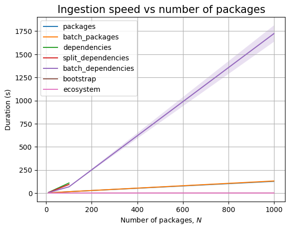
One more database to look at, so let’s go.
NebulaGraph 🔗
One nice part about NebulaGraph’s documentation is that they present a comprehensive history of graph databases but also fully document everything, starting from architecture.
Similar to TerminusDB, we have to clone a repository to set up Docker:
[...]$ git clone -b release-3.4 https://github.com/vesoft-inc/nebula-docker-compose.git
[...]$ cd nebula-docker-compose/
[...]$ docker-compose up
The Python client is not available in NixOS, so we need to createa shell for it, like we did for TerminusDB:
{ pkgs ? import <nixpkgs> {} }:

let
  local_nebula = ps: with ps; [
    (
      buildPythonPackage rec {
        pname = "nebula3-python";
        version = "3.4.0";
        src = fetchPypi {
          inherit pname version;
          sha256 = "sha256-R72LG0uywvDlEivBR5JstQV4pmhBrPanQ8rk0DYsnqo=";
        };
        doCheck = false;
        buildInputs = [
          future
          httplib2
        ];
        propagatedBuildInputs = [
          pytz
          six
        ];
      }
    )
  ];
in
  with pkgs;
  mkShell {
    nativeBuildInputs = [
      (python311.withPackages local_nebula)
    ];

    shellHook = ''
      export PS1="[\[\033[01;32m\]nix-shell\[\033[00m\]:\W] \[\033[01;32m\]λ\[\033[00m\] "
    '';
  }
Unfortunately, the Python client documentation is not as complete. But, the query syntax is very similar to what we have seen so far in ArangoDB and Neo4j, so I can guess how to write them.
In NebulaGraph we need to define the vertex IDs manually.
Hence, we will use the same pattern as in ArangoDB where we encode the node
contents into its ID. This is helpful, since there is no support for
Neo4j’s MERGE and since inserting a node
with the same ID and label overwrites the properties corresponding to that
label.
The last phrase will be easier to understand once we realize that NebulaGraph is schema first: each node label (called tag) defines the list of properties that the node should contain (and developers should minimize the number of times the tag definition gets altered). The entire schema is collected into a space, so we need to create a space to operate on data instead of using the default one. Fortunately, we can quickly delete all data by deleting the space.
Thus, we can write the following code:
class NebulaGraph(Experiment):
    def __init__(self, N: int, B: int, K: int, shuffle: bool = True, threaded: bool = True):
        super().__init__(N, B, K, shuffle, threaded)
        import nebula3
        from nebula3.gclient.net import ConnectionPool
        from nebula3.Config import Config
        self._cp = ConnectionPool()
        self._cp.init([('127.0.0.1', 9669)], Config())
        self._client = self._cp.get_session('root', 's3cr3tp455')
        self._sleep_time = 11

    def __del__(self):
        self._client.release()
        self._cp.close()

    def setup(self, indexes: bool = True):
        script = """
CREATE SPACE IF NOT EXISTS test(vid_type=FIXED_STRING(8));
USE test;
CREATE TAG IF NOT EXISTS ecosystem();
CREATE TAG IF NOT EXISTS namespace();
CREATE TAG IF NOT EXISTS name();
CREATE TAG IF NOT EXISTS version();
CREATE TAG IF NOT EXISTS dependency();
CREATE EDGE IF NOT EXISTS has_namespace();
CREATE EDGE IF NOT EXISTS has_name();
CREATE EDGE IF NOT EXISTS has_version();
CREATE EDGE IF NOT EXISTS has_dependency();
CREATE EDGE IF NOT EXISTS has_target();
CREATE TAG INDEX IF NOT EXISTS I1 ON ecosystem();
CREATE EDGE INDEX IF NOT EXISTS I7 ON has_version();
"""
        self._client.execute(script)
        time.sleep(self._sleep_time)

        if indexes:
            pass

    def _do_clean(self):
        self._client.execute('DROP SPACE test')

    # ...
It is important to note that we always create two indexes in setup and
ignore the value of indexes argument. This is because queries return an
error if they would require a database scan without a limit or an index
present. The two indexes included here are the minimal ones needed to be able
to run all experiments. It turns out we don’t need others, and anyway
documentation warns us to be careful with indexes because using them
can slow down ingestion (and we have already seen this in
the Neo4j case).
One significant issue here is that we need to sleep at the end of setup
to make sure that all the schema definition is valid before we start
ingesting. This will result in a slow-down for our experiments. But a much
larger figure is that the sleep time is not documented, so I picked a value
that allowed me to run all experiments.
For clean-up, we cannot just delete all nodes and edges because deletion is not atomic. Fortunately, we can just delete the entire space.
Moving towards ingestion, we have two constraints: UPSERT should not be
used in threaded scenarios and UNWIND only works
inside a query. The first one is just another hint that we
should just use INSERT, whereas the second one will impact batch ingestion:
class NebulaGraph(Experiment):
    # ...

    def _do_ingest_package(self, package: Package):
        ecosystem = f'e_{package.ecosystem}'
        namespace = f'{package.ecosystem}_{package.namespace}'
        name = f'{namespace}_{package.name}'
        version = package.version

        query = f"""
INSERT VERTEX ecosystem() VALUES "{ecosystem}":();
INSERT VERTEX namespace() VALUES "{namespace}":();
INSERT VERTEX name() VALUES "{name}":();
INSERT VERTEX version() VALUES "{version}":();
INSERT EDGE has_namespace() VALUES "{ecosystem}"->"{namespace}":();
INSERT EDGE has_name() VALUES "{namespace}"->"{name}":();
INSERT EDGE has_version() VALUES "{name}"->"{version}":();
"""
        self._client.execute(query)

    def _do_ingest_batch_packages(self, packages: Sequence[Package]):
        for package in packages:
            self._do_ingest_package(package)

    # ...
Dependencies can be ingested in a similar fashion:
class NebulaGraph(Experiment):
    # ...

    def _do_ingest_dependency(self, dependency: Dependency):
        parent = dependency.parent.version
        target = dependency.target.version
        dependency = f'dep_{parent}-{target}'

        query = f"""
INSERT VERTEX dependency() VALUES "{dependency}":();
INSERT EDGE has_dependency() VALUES "{parent}"->"{dependency}":();
INSERT EDGE has_target() VALUES "{dependency}"->"{target}":();
"""

        self._client.execute(query)

    def _do_ingest_batch_dependencies(self, dependencies: Sequence[Dependency]):
        for dependency in dependencies:
            self._do_ingest_dependency(dependency)

    # ...
Finally, for the queries, we can just use the same pattern as in the Neo4j case, with the names changed and making sure we have the required indexes:
class NebulaGraph(Experiment):
    # ...

    def _do_query_bootstrap(self):
        query = """
MATCH (a:version) <-[:has_version]- (:name) -[:has_version]-> (b)
                  -[:has_dependency]-> (:dependency) -[:has_target]-> (a)
RETURN id(b) AS parent, id(a) AS target
"""
        response = self._client.execute(query)
        if not response.is_succeeded():
            print(response.error_msg())
            return []
        ret = []
        for record in response:
            parent, target = record.values()
            ret.append((parent.as_string(), target.as_string()))
        return ret

    def _do_query_ecosystem(self):
        query = """
MATCH (e1:ecosystem)
MATCH (e2:ecosystem)
WHERE e1 <> e2
MATCH (e1) -[:has_namespace]-> (:namespace) -[:has_name]-> (:name) -[:has_version] -> (v1:version)
MATCH (e2) -[:has_namespace]-> (:namespace) -[:has_name]-> (:name) -[:has_version] -> (v2:version)
MATCH (v1) -[has_dependency]-> (:dependency) -[has_target]-> (v2)
RETURN id(v1) AS parent, id(v2) AS target
"""
        response = self._client.execute(query)
        if not response.is_succeeded():
            print(response.error_msg())
            return []
        ret = []
        for record in response:
            parent, target = record.values()
            ret.append((parent.as_string(), target.as_string()))
        return ret
We need a little bit more work to parse the returned data, but this is not something complex.
We can now move to run the experiments. We already know that -i flag is not
needed since we are forced to use indexes. Turns out that here too there are
some issues with threading, as in my experiments I’ve been seeing frequent
deadlocks. Hence, we won’t use threads here either.
With that being said, here’s the data:
| Experiment | type | time (s) | stddev (s) |
|---|---|---|---|
packages |
28.345 | ±0.048 | |
| shuffled | 28.245 | ±0.090 | |
batch_packages |
28.269 | ±0.039 | |
| shuffled | 28.202 | ±0.083 | |
dependencies |
326.836 | ±0.315 | |
| shuffled | 326.119 | ±0.414 | |
split_dependencies |
210.490 | ±0.145 | |
| shuffled | 210.322 | ±0.237 | |
batch_dependencies |
66.158 | ±0.049 | |
| shuffled | 66.139 | ±0.098 |
There is no difference between shuffling the data or not. We can see the same in the plot:
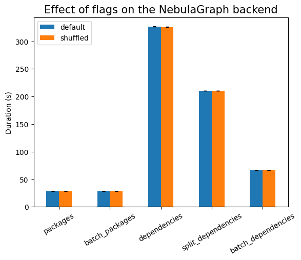
Moving on to \(N\), we see the usual linear increase:
| Experiment | N | time (s) | stddev (s) |
|---|---|---|---|
packages |
10 | 0.039 | ±0.010 |
| 100 | 0.294 | ±0.004 | |
| 1000 | 2.828 | ±0.043 | |
| 10000 | 28.245 | ±0.090 | |
| 100000 | 286.106 | ±0.357 | |
batch_packages |
10 | 0.037 | ±0.009 |
| 100 | 0.327 | ±0.142 | |
| 1000 | 2.769 | ±0.097 | |
| 10000 | 28.202 | ±0.083 | |
| 100000 | 284.925 | ±0.231 | |
dependencies |
10 | 0.312 | ±0.044 |
| 100 | 3.358 | ±0.132 | |
| 1000 | 32.588 | ±0.121 | |
| 10000 | 326.119 | ±0.414 | |
split_dependencies |
10 | 0.238 | ±0.013 |
| 100 | 2.207 | ±0.033 | |
| 1000 | 21.103 | ±0.072 | |
| 10000 | 210.322 | ±0.237 | |
batch_dependencies |
10 | 0.113 | ±0.004 |
| 100 | 0.848 | ±0.033 | |
| 1000 | 6.756 | ±0.037 | |
| 10000 | 66.139 | ±0.098 | |
| 100000 | 664.936 | ±3.385 | |
bootstrap |
10 | 0.037 | ±0.065 |
| 100 | 0.007 | ±0.000 | |
| 1000 | 0.030 | ±0.002 | |
| 10000 | 0.740 | ±0.026 | |
ecosystem |
10 | 0.015 | ±0.001 |
| 100 | 0.031 | ±0.001 | |
| 1000 | 0.706 | ±0.005 |
Not many ingestion methods reach large values of \(N\), so the lines are trimmed early:
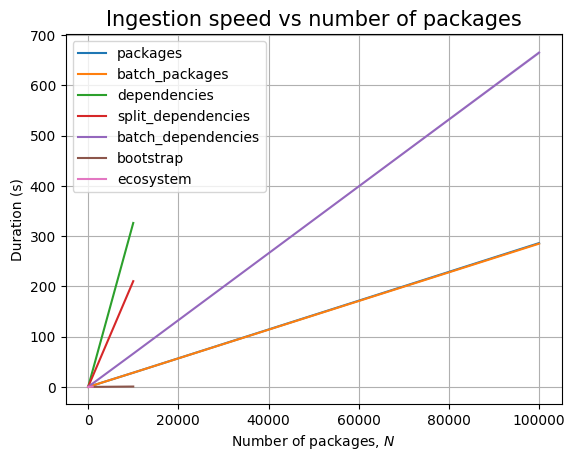
However, we can zoom in to the span where we have all methods:
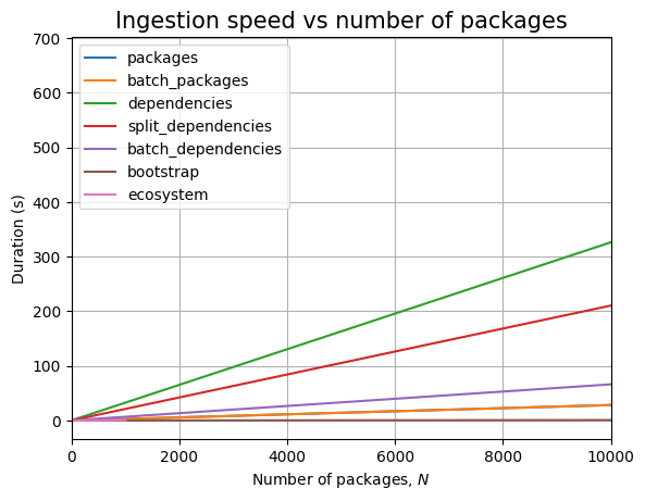
And we can also just focus on the queries:
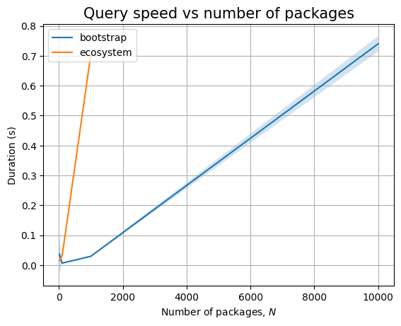
We have the same similar pattern, bootstrap queries are faster than ecosystem ones.
Let’s look at the results of testing the dependency on \(B\):
| Experiment | B | time (s) | stddev (s) |
|---|---|---|---|
packages |
2 | 28.309 | ±0.240 |
| 4 | 28.206 | ±0.071 | |
| 8 | 28.252 | ±0.040 | |
batch_packages |
2 | 28.133 | ±0.074 |
| 4 | 28.239 | ±0.146 | |
| 8 | 28.196 | ±0.094 | |
dependencies |
2 | 324.684 | ±0.261 |
| 4 | 325.863 | ±0.527 | |
| 8 | 326.628 | ±0.398 | |
split_dependencies |
2 | 209.831 | ±0.166 |
| 4 | 210.702 | ±0.228 | |
| 8 | 210.787 | ±0.288 | |
batch_dependencies |
2 | 66.078 | ±0.138 |
| 4 | 66.229 | ±0.082 | |
| 8 | 66.050 | ±0.147 | |
bootstrap |
2 | 10.511 | ±0.131 |
| 4 | 1.327 | ±0.022 | |
| 8 | 0.257 | ±0.005 |
Everything seems constant, except the bootstrap query that seems to be affected by consistently biased node for \(B=2\).
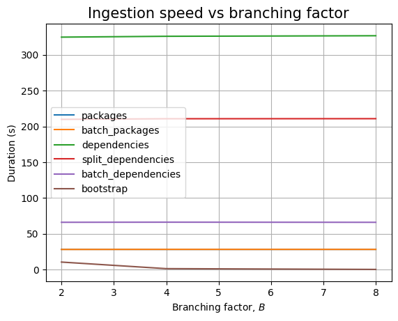
Note that ecosystem queries run out of memory for 10k packages, hence we cannot study how they are affected by \(B\).
| Experiment | K | time (s) | stddev (s) |
|---|---|---|---|
dependencies |
1 | 65.074 | ±0.086 |
| 2 | 130.195 | ±0.192 | |
| 4 | 261.340 | ±0.417 | |
| 8 | 522.725 | ±0.370 | |
split_dependencies |
1 | 65.085 | ±0.077 |
| 2 | 101.504 | ±0.061 | |
| 4 | 174.510 | ±0.047 | |
| 8 | 320.130 | ±0.274 | |
batch_dependencies |
1 | 35.895 | ±0.120 |
| 2 | 43.459 | ±0.118 | |
| 4 | 58.552 | ±0.071 | |
| 8 | 89.176 | ±0.271 | |
bootstrap |
1 | 0.669 | ±0.005 |
| 2 | 0.682 | ±0.011 | |
| 4 | 0.690 | ±0.005 | |
| 8 | 0.728 | ±0.008 |
Finally, \(K\) has the expected linear effect.
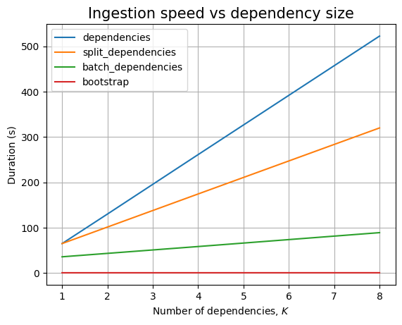
We can also zoom in for the bootstrap query since that looks nearly constant:
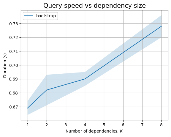
Modulo noise, it actually also increases linearly.
And this concludes the study of all 6 databases. It is time for cross database comparisons and final conclusions.
Results 🔗
We can begin by doing a scatter point of each database engine on the 4 query types we care about: ingesting packages, ingesting dependencies, querying for bootstrap patterns and querying for cross ecosystem dependencies.
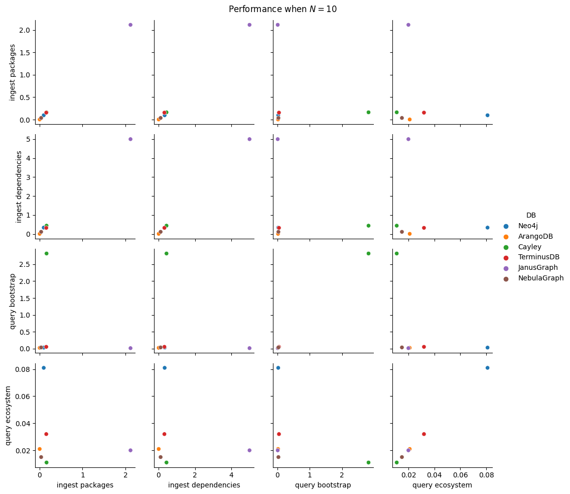
In each of these scatter plots, we have one point for each dataset, with an associated hue.
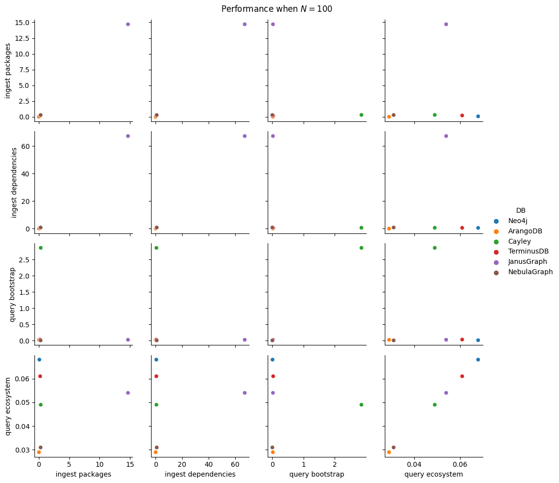
If the dataset cannot support a given value of \(N\), there is no point being displayed.
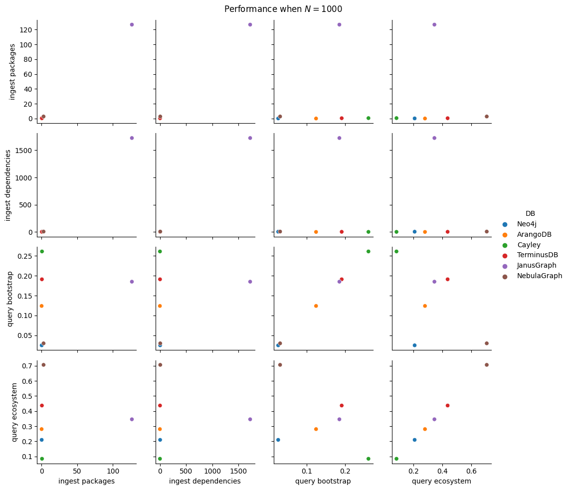
For each of the 4 query types, we select the minimum average time. That is, between the two ingestion methods for packages, in general we’d select the batch ingestion except the cases where it is either similar to the regular one or it results in an error.
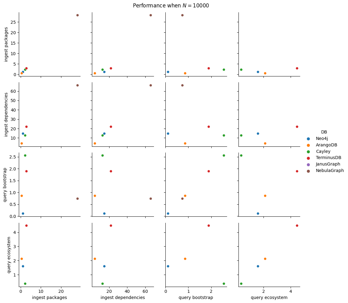
We do a similar thing for the 3 different dependency ingestion methods.
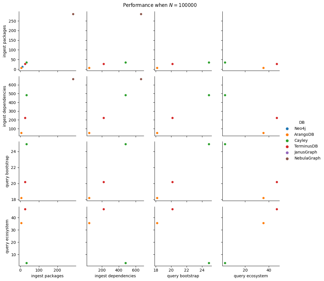
For the queries themselves, there’s only one set of data points, and that is the one we are considering.
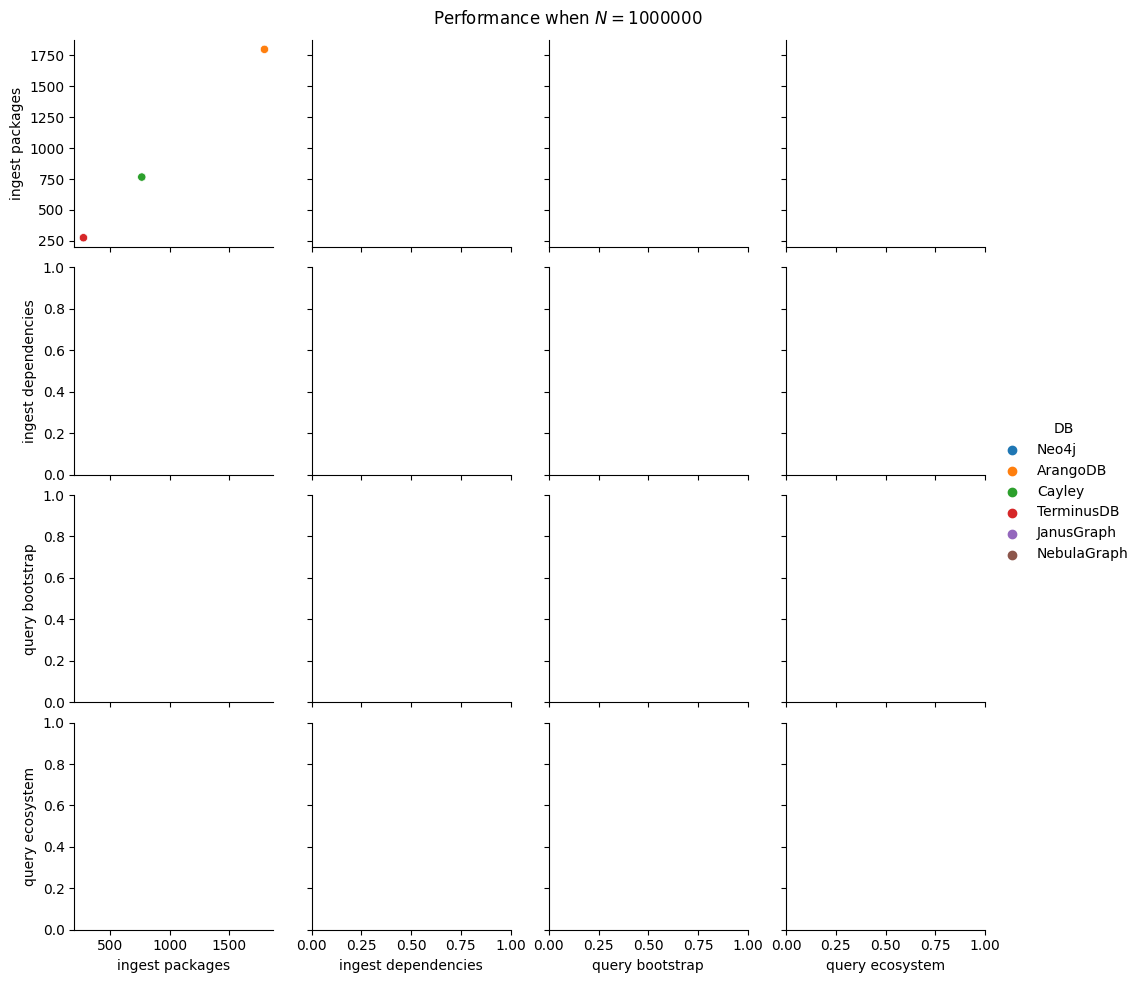
Ideally, looking at time only, we’d prefer the databases that are closest to origin in most of these plots. Alternatively, we can see that there are databases that are better suited for reading the data and databases that have strong performance on ingestion. Since I know people want to see winners, by either metric, it seems that ArangoDB is a clear winner, followed closely by NebulaGraph and Neo4j. Cayley wins several rounds due to the inversion between bootstrap and ecosystem queries.
Overall, we are able to ingest 1 million packages with ArangoDB, Cayley, and TerminusDB, but no backend is able to ingest 1 million dependencies in the allotted time frame. Sure, we have to fallback to regular ingestion in a few cases, as the batch size results in OOM errors, but this gives us a suggestion that we can ingest in smaller batches and still achieve good performance. This approach might apply for ingesting 1 million dependencies too, but that’s left for testing for later.
Moving beyond speed, the 6 databases that I’ve tests have various levels of support and polish. Some have extensive documentation, others have extensive stories about the need for graph databases but lack exactly the documentation that is needed to use them. Some databases come with an integrated visualizer and the UX also allows for efficient profiling of queries, whereas others rely more on reading the documentation (as much as it is) and experimenting. Some of these are easy to use, just a single docker container with no additional setup and configuration, others require multiple steps of preparation.
Query readability also differs significantly between the 6 databases. On the one hand, this is expected, given that these are using different base principles. We cannot expect queries in RDF world to match queries in document store backends world.
Overall, this has been a very productive month. I have learned these 6 databases (and ones that are similar) to sufficient levels to run these benchmarks. It is very possible that I have missed some optimizations, some ways of writing more performant queries. Happy to fix these and run new benchmarks, if you send some comments. Similarly, if you think there are other databases to test, please leave a comment.
There are a bunch of follow-up items left in this post already. I will write a new post soon with them (most importantly, with the path queries – but only for some of the databases, I’ll exclude some that didn’t pass these tests). But first, I’m quite late in publishing other drafts, including new installments on the VDGF series. Stay tuned :)
PS: I have learned a lot about experimental design too, from this post and the previous one. I now know to estimate an upper bound of total experiment time before heading in the work, create contingency plans and push the data into a (SQL :P) database from which scripts can read it and automatically generate the tables and plots to include in the post. Future benchmarks (if I do more), will be faster and in shorter articles. This gargantuan should be a singleton.
The
hasboltpackage was last updated in 2022 and only supports version 3. All other packages are older.↩︎Commercial license required for most features↩︎
There is an official Python repository but with no PyPI release (thus, not in NixOS) and a community built Python Package which is old, not available for modern Python versions, and only tied to an old version of Cayley. Both are no longer updated :(↩︎
The
cayley-clientpackage was last updated in 2022 and only supports version 0.3.↩︎Client is not the official client for JanusGraph, only works due to underlying query language matching↩︎
Similarly, there is no specific Python client, we have to use TinkerPop’s Python client. The Python repository never contained any real code.↩︎
Here too, we have generic package to Gremlin/TinkerPop↩︎
CC-BY license only for documentation after 2016 fork, Apache2 for documentation before the fork↩︎
Only the TinkerPop client exists.↩︎
This could have been done in
__init__(RAII), but I realized this much later, so I decided to not alter the code anymore.↩︎After running all experiments, I realized during data processing, that this could have been done better: put the data in a SQL table or something and write a script that selects only the corresponding rows. Lesson learned for future similar experiments.↩︎
At some point, if I continue doing such experiments, I’ll need to invest on a separate system just for running these. Perhaps in the cloud? Though those could be labelled as mining crypto and I could get banned :|↩︎
For the other database backends we identify the version node with the pURL directly, given that the other databases are not really graph-first. In a future article, I might retry the Neo4j examples assuming the same mapping.↩︎
Comments:
There are 9 comments (add more):