A last look at Silksong (for now)

I already posted two separate articles on how to use math to do a better decision regarding conserving the in-game currency in Silksong, given that many players need a lot of attempts before they git gud. This is the last one, and here we are actually modelling how players are getting better at each stage of the game, the more and more they play it, rather than throw away the console in frustration.

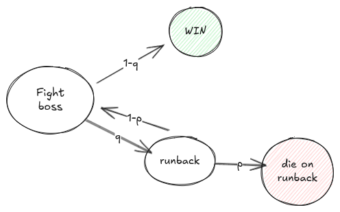
In the last article we used \(q\) to model the probability that the player dies when fighting a boss or navigates a difficult parkour section, and \(p\) as the probability to die on the runback, before recovering their currency. That is, we had these events:

1. win the boss on first fight (with probability \(1-q\))
2. lose on the first fight (with probability \(q\)) and then
   1. die on runback, losing money (with probability \(p\))
   2. reach the boss again (with probability \(1-p\)) and then repeat this scenario

Which we also represented as a state machine:

However, in this model we assumed that the player has the same chances as in the first attempt, even if they are attempting the same thing for the 23424th time, in an attempt to prove false that classical definition of insanity.

In practice, though, the more attempts a player does, the lower the chance that they fail. We want something like this:

That is, each new attempt is exponentially better than the previous one, when I’m using the colloquial meaning here.

Actually, the attempts are discrete, so we won’t get a curve, but a collection of points that are smaller and smaller. And, for simplicity, let’s assume that the actual probability is a Poisson Distribution. We have to pick the rate parameter between 0 and 1, to simulate a probability that is always going lower:

So, let’s assume that the value of \(q\) on the \(k\) attempt is

\(q_k = \frac{\lambda^k e^{-\lambda}}{k!}\)

And, similarly, the value of \(p\) on the \(k\) attempt is

\(p_k = \frac{\mu^k e^{-\mu}}{k!}\)

That is, we replaced the two parameters \(p\) and \(q\) from the previous article with the \(\lambda\) and \(\mu\) parameters of the distributions (which both should be between 0 and 1).

Looking back at the state machine, we can write the same probabilities as in the last article:

• The probability to end in the green state is:

\[P_w = \left(1-q_1\right) + q_1\left(1-p_1\right)\left(1-q_2\right) + q_1q_2\left(1-p_1\right)\left(1-p_2\right)\left(1-q_3\right) + \ldots\]

• The probability to end on the red, bad state is:

\[P_r = q_1p_1 + q_1q_2\left(1-p_1\right)p_2 + q_1q_2q_3\left(1-p_1\right)\left(1-p_2\right)p_3 + \ldots\]

These can no longer be reduced as simple as in the previous article. In fact, I don’t know of any other way to get simpler formulas except by numerical methods. The product of \(q\) factors can be reduced to a fraction that has a product of factorials as it denominator, but the product of the \(1-p\) factors gets much more complicated to ever hope we can get some closed form formula.

Perhaps I made the model too complicated. In the end, each model is useful as long as it is not that complex that it no longer makes predictions. The model from the previous two articles is already quite useful, we don’t need to overcomplicate like here. Just because we can, it doesn’t mean we should… Let’s just play the game.