Evolving isDigit

I had other plans for this weekend but I got nerd-snipped (obligatory xkcd reference) due to some coincidences. First, during the week, Nick was talking about using bit operations and Karnaugh maps to implement isAscii. Then, today, Dorin was looking for a way to implement isDigit in a similar way.

Being so primed, I started doing the usual logical expression minimization and trying to find the expression that would work here. However, in the middle of it I had a different idea: what if we ask the computer to come up with the function?.

Setup 🔗

This is not about asking ChatGPT to solve the issue, nor is this trying to use neural networks like in a famous article. Instead, we’ll be using genetic algorithms. As usual, I’ll be using Haskell. Starting with a new empty file, let’s add the following shebang (so that we can run cabal run without having a Cabal file) and imports:

#!/usr/bin/env cabal
{- cabal:
build-depends: base, mtl, random
-}

import Control.Monad.State
import Data.Bits hiding (And, Xor)
import Data.Char
import Data.List
import Data.Word
import System.Random
import Text.Printf

Both Dorin and Nick were talking about char types in C/C++, so we will be working a lot with Word8 in Haskell. Genetic algorithms imply a lot of randomness and we will be using helpers from the other imports in some places.

The fastest working implementation would be

bool isDigit(char c) {
    return (unsigned char)(c - '0') < 10;
}

In Haskell, this translates almost without any changes:

testIsDigit :: Word8 -> Bool
testIsDigit c = c - (fromIntegral $ ord '0') < 10

We want to write some code to make the computer come up with a function from Word8 to Bool which would return the exact same values as testIsDigit for all 256 values of the Word8 type.

The expressions 🔗

We want to only use bit operations. We need to add the logical negation though, to be able to convert values that have a bit set to logical values.

Thus, we can define our expression type:

data Expr
  = Var
  | Val Word8
  | Not Expr
  | Complement Expr
  | And Expr Expr
  | Or Expr Expr
  | Xor Expr Expr
  deriving (Eq, Show)

The Var constructor is a standin for the input character, whereas Val will be used to introduce constants. We use Not to denote the logical not operator (not in Haskell, ! in C/C++) and Complement to denote flipping all bits of the argument expression. And then, we have the 3 common bitwise operations.

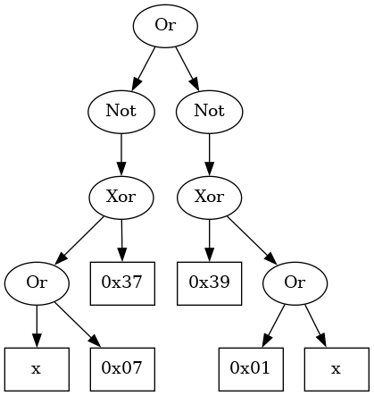
Our goal is to have a genetic algorithm grow trees based on this expression type. Each tree represents a possible implementation of isDigit. For example, the following tree represents the desired solution (modulo ordering of the children):

We need to evaluate these trees. We do this in several stages. First, given an expression tree and an input argument, let’s determine what is the value that the tree computes at that argument:

evalAt :: Expr -> Word8 -> Word8
evalAt Var x = x
evalAt (Val v) _ = v
evalAt (Not e) x = if evalAt e x /= 0 then 0 else 1
evalAt (Complement e) x = complement $ evalAt e x
evalAt (And e1 e2) x = (evalAt e1 x)  .&.  (evalAt e2 x)
evalAt (Or  e1 e2) x = (evalAt e1 x)  .|.  (evalAt e2 x)
evalAt (Xor e1 e2) x = (evalAt e1 x) `xor` (evalAt e2 x)

Nothing too fancy, we return the input for Var, propagate constants for Val, and evaluate the children nodes before combining them for the other cases. Of particular interest here is the Not case: evaluating this node must return only 0 or 1 (in truth, only False or True but we’ll leave this conversion for later).

Now that we know what an expression evaluates at a specific point, we can compare with the result of testIsDigit at the same argument:

testAt :: Expr -> Word8 -> Bool
testAt e x
  | testIsDigit x = evalAt e x /= 0
  | otherwise = evalAt e x == 0

If testIsDigit x returns True we want evalAt e x to also return a true-ish (as per C/C++ convention) value. If testIsDigit x returns False, then evalAt e x must return 0 (the only False value).

As an exercise for the reader, consider why the following implementation would be incorrect:

testAtBad :: Expr -> Word8 -> Bool
testAtBad e x = testIsDigit x == evalAt e x

The only remaining thing to do here is to test the expression tree across the entire range:

test :: Expr -> Int
test e = length $ filter (testAt e) allChars
  where
    allChars = [minBound..]

We just return the number of instances where the two functions match. For a perfect implementation, this should be equal to the cardinality of the Word8 type, that is, 256. And, indeed, our expression represented in the above image performs as expected:

ghci> test (Or (Not $ Xor (Val 0x37) $ Or Var (Val 0x07)) (Not $ Xor (Val 0x39) $ Or Var (Val 0x01)))
256

With the evaluation out of the way, it is time to move to the next step: defining the genetic algorithm.

The Evolution of Trees 🔗

A genetic algorithm initializes a random collection of objects that encode some problem (i.e., in our case, the Expr trees) and then, over a certain number of iterations, operates on these structures trying to optimize a scoring function (i.e., in our case, the result of test). Each iteration involves combining elements of the collection and slightly altering them, in a non-deterministic way.

The above short summary is not unique to genetic algorithms. Instead, a wide range of so called evolutionary algorithms follow the same strategy, differing only in the ordering and the implementation of the operations. Perhaps in the future, I will go into more details on these algorithms, solving relevant problems. But for now, let’s implement a naïve genetic algorithm.

Initializing the population 🔗

We need to grow multiple trees randomly, to start the exploration. Since we have an inductive data structure, it is possible for the generation to never terminate – though with vanishing probabilities, if all possible trees are equally likely. However, here we use a much simpler tree generation scheme: we pick a random number to select the constructor and then we generate the children subexpressions as needed. Thus, in order to not go into cases where the trees are too large, or the generation does not finish, we also impose a maximum tree depth. From the above image we know that a tree of depth 5 should suffice, but let’s give the algorithm a larger search space:

gMaxDepth :: Int
gMaxDepth = 15

genRandomExpr :: State StdGen Expr
genRandomExpr = go 0
  where
    go depth = do
      branch <- state $ randomR (0 :: Int, if depth > gMaxDepth then 2 else 6)
      case branch of
        0 -> return Var
        1 -> Val <$> state random
        _ -> do
          e1 <- go $ depth + 1
          case branch of
            2 -> return $ Not e1
            3 -> return $ Complement e1
            _ -> do
              e2 <- go $ depth + 1
              case branch of
                4 -> return $ And e1 e2
                5 -> return $ Or e1 e2
                _ -> return $ Xor e1 e2

If the tree reaches the maximum depth, we only generate Var and Val nodes, otherwise we need to generate at least one subexpression. For the binary operations, we have the most nested case, after generating the second subexpression.

Now that we have a random tree generator, using State monad to keep track of the random generator for us, we can generate the entire initial population:

gPopulationSize :: Int
gPopulationSize = 100000

genInitialTrees :: State StdGen [Expr]
genInitialTrees = replicateM gPopulationSize genRandomExpr

Now that we have this (quite large) population, we can run the evolution algorithm.

One evolution round 🔗

Let’s assume that at the beginning of each evolution round we look at each tree in our population, evaluate it (using test) and then sort our population in descending order of this score (also known as fitness). We define a helper function for this:

sortExpressions :: [Expr] -> [Expr]
sortExpressions = sortOn (negate . test)

Here, I’m using the point-free style (also known as pointless, as a joke): the argument of the function is not written explicitly, but instead the entire expression uses function composition. Using negate makes the expressions with the higher score be sorted earlier, without needing to resort to using reverse to reverse an increasing list into decreasing order.

With this helper, we can define our genetic algorithm round. For each round, we start with a sorted list of expression trees, keep the best performing one (the first one) and then use this list to generate the remaining elements for the next round: we select 2 individuals from the population, and merge them to create 2 new trees. These trees will be potentially nudged to introduce new features and then added back to the population. Overall, the code looks like this:

gaRound :: Int -> [Expr] -> State StdGen Expr
gaRound 0 (e:_ ) = return e
gaRound n (e:es) = do
  let
    fitness = map test es
    summed = scanl1 (+) fitness
    roulette = zip es summed
    total = last summed
  new <- replicateM (gPopulationSize - 1) $ do
    a <- selectFromPopulation total roulette
    b <- selectFromPopulation total roulette
    (a', b') <- cross a b
    a'' <- mutate a'
    b'' <- mutate b'
    return [a'', b'']
  gaRound (n - 1) (take gPopulationSize $ sortExpressions $ e:concat new)

If we reach round 0, we return the first tree, as that is supposed to be the best performer. Otherwise, we repeat the process mentioned above, for a total of gPopulationSize - 1 rounds. in each round we get 2 new children, so after we sort all the 1 + 2 * (gPopulationSize - 1) nodes, we take only the first gPopulationSize ones. This means that even if we kept aside the best performer from the previous generation, if enough new children have a better fitness this old node will be removed.

All that is left to do is to describe the 3 operations: selecting individuals to combine, performing the actual recombination and performing the mutation.

Random selection 🔗

To select the individuals to reproduce, we give more chances to those that have a higher fitness. This is why in summed we keep a prefix sum of all fitnesses, which we then zip in roulette. For 4 individuals, e1, e2, e3, and e4, with fitnesses 100, 50, 25 and 25, we have

-- roulette = [(e1, 100), (e2, 150), (e3, 175), (e4, 200)]

That is, in graphical form:

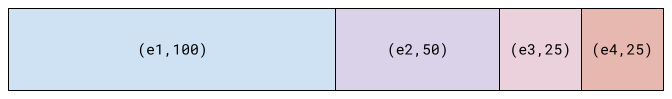
Now, we just through a dart at the above diagram and select the individual that corresponds to the rectangle where the dart lands. Or, in code:

selectFromPopulation :: Int -> [(Expr, Int)] -> State StdGen Expr
selectFromPopulation max scoredExprs = do
  dart <- state $ randomR (0, max - 1)
  return $ go dart scoredExprs
    where
      go x ((e,s):es)
        | x > s = go x es
        | otherwise = e

In the go helper, we keep removing rectangles from the start of the diagram until we find the one with the dart.

Crossover 🔗

Given 2 trees, how do we combine them? The idea is simple: pick a subtree in each of the 2 individuals and then swap these around. Similar to the following picture:

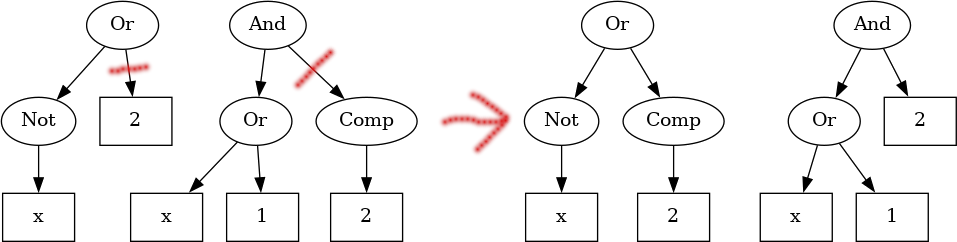
In code, this is slightly more complex. Rather than doing everything all at once, let’s go step by step.

First, let’s just determine how big a tree is, that is, how many nodes it has. This is a simple recursive function, pattern matching on each constructor:

exprSize :: Expr -> Int
exprSize Var = 1
exprSize (Val _) = 1
exprSize (Not e) = 1 + exprSize e
exprSize (Complement e) = 1 + exprSize e
exprSize (And e1 e2) = 1 + exprSize e1 + exprSize e2
exprSize ( Or e1 e2) = 1 + exprSize e1 + exprSize e2
exprSize (Xor e1 e2) = 1 + exprSize e1 + exprSize e2

In the above imagine, the first tree would have size 4, whereas the second would have size 6.

Now that we have the sizes of both expressions, we can pick a random number between 0 and the minimum size and that would give us the node that needs to be swapped. Assuming we have this number, let’s compute this subtree:

getSubExprAt :: Expr -> Int -> Expr
getSubExprAt e 0 = e
getSubExprAt e@Var _ = e
getSubExprAt e@(Val _) _ = e
getSubExprAt   (Not        e) x = getSubExprAt e (x - 1)
getSubExprAt   (Complement e) x = getSubExprAt e (x - 1)
getSubExprAt   (And e1 e2) x =
  let s = exprSize e1 in
  if s > x then getSubExprAt e1 x else getSubExprAt e2 (x - s)
getSubExprAt   (Or  e1 e2) x =
  let s = exprSize e1 in
  if s > x then getSubExprAt e1 x else getSubExprAt e2 (x - s)
getSubExprAt   (Xor e1 e2) x =
  let s = exprSize e1 in
  if s > x then getSubExprAt e1 x else getSubExprAt e2 (x - s)

It is again a recursive function, matching on each constructor. If the number of nodes left to traverse reaches 0 we return the current node. For variables or constants, we also don’t descend further. For the binary nodes, we compute the size of the left children and descend only in the node that is relevant.

Finally, if we have a tree, an index where a replacement needs to be inserted and the replacement, we can perform this operation:

placeAt :: Expr -> Int -> Expr -> Expr
placeAt _ 0 r = r
placeAt Var     _ r = r
placeAt (Val _) _ r = r
placeAt (Not        e) n r = Not        $ placeAt e (n - 1) r
placeAt (Complement e) n r = Complement $ placeAt e (n - 1) r
placeAt (And e1 e2) n r =
  let s = exprSize e1 in
  if s > n then And (placeAt e1 n r) e2 else And e1 (placeAt e2 (n - s) r)
placeAt (Or  e1 e2) n r =
  let s = exprSize e1 in
  if s > n then Or  (placeAt e1 n r) e2 else Or  e1 (placeAt e2 (n - s) r)
placeAt (Xor e1 e2) n r =
  let s = exprSize e1 in
  if s > n then Xor (placeAt e1 n r) e2 else Xor e1 (placeAt e2 (n - s) r)

Just like above, if the index is 0 then we replace the current node. We do the same if the current node is a leaf (Var/Val). In principle, placeAt and getSubExprAt follow the same recursion scheme.

With these pieces in place, we can write the crossover operator:

cross :: Expr -> Expr -> State StdGen (Expr, Expr)
cross e1 e2 = do
  let
    s1 = exprSize e1
    s2 = exprSize e2
    sz = min s1 s2
  r <- state $ randomR (0, sz - 1)
  return
    ( placeAt e1 r $ getSubExprAt e2 r
    , placeAt e2 r $ getSubExprAt e1 r
    )

It goes exactly as described: we compute the sizes, pick a random index, extract the subtrees at those nodes and swap them around. This completes the image from the start of this section.

But we need one more operation to have the genetic algorithm work.

Mutation 🔗

With all we have defined so far, the constants that are generated at the beginning of the program during genInitialTrees will be the only ever that the algorithm considers. Similarly, most of the structure will stay the same as it was after the initial generation round.

To introduce some diversity in the population, we need to mutate the trees. We don’t want to mutate all of them as mutations can as well destroy useful information. So, we introduce a mutation probability to gate the process:

gMutateProba :: Float
gMutateProba = 0.1

The mutation is relatively simple: the Var node cannot migrate anywhere (since we have only one variable), the Val node will have the constant nudged by one unit up or down. The unary constructors would swap, whereas the binary ones would cycle:

mutate :: Expr -> State StdGen Expr
mutate e = do
  r <- state random
  if r > gMutateProba
  then return e
  else case e of
    Var -> return Var -- nothing to change
    -- swap
    Not e'        -> return $ Complement e'
    Complement e' -> return $ Not e'
    _ -> do
      up <- state random
      case e of
        Val x -> return $ Val (if up then x + 1 else x - 1)
        -- cycle
        And e1 e2 -> return $ if up then  Or e1 e2 else Xor e1 e2
        Or e1 e2  -> return $ if up then Xor e1 e2 else And e1 e2
        Xor e1 e2 -> return $ if up then And e1 e2 else  Or e1 e2

This is enough to generate diversity.

Putting it all together 🔗

Now, all we need to do is run several rounds of the genetic algorithm and benefit from the fact that the individuals with higher fitness have higher chances of survival and combination:

gNumRounds :: Int
gNumRounds = 10000000

ga :: State StdGen Expr
ga = do
  initial <- sortExpressions <$> genInitialTrees
  gaRound gNumRounds initial

In our main function we only need to call ga, given an initilized random number generator and evaluate the State.

main :: IO ()
main = do
  expr <- evalState ga <$> initStdGen
  printf "Best score %d\n" $ test expr
  printf "Best expression %s\n" $ pPrint expr

There is only remaining item. Our Expr type implements Show but the resulting expression is harder to read. So, we can implement a pretty-printer to better display the result:

pPrint :: Expr -> String
pPrint Var = "x"
pPrint (Val v) = show v
pPrint (Not e) = printf "!(%s)" $ pPrint e
pPrint (Complement e) =  printf "~(%s)" $ pPrint e
pPrint (And e1 e2) = printf "(%s) & (%s)" (pPrint e1) (pPrint e2)
pPrint (Or  e1 e2) = printf "(%s) | (%s)" (pPrint e1) (pPrint e2)
pPrint (Xor e1 e2) = printf "(%s) ^ (%s)" (pPrint e1) (pPrint e2)

This is just traversing the tree node by node and combining the results of the recursive calls. In fact, it is very similar to evalAt, the first function we’ve written in this article. And this is not a coincidence: whereas evalAt evaluates a tree to a Word8, pPrint evaluates it to a String. Thus, they use the same recursion scheme. I’m planning to expand on this in the future.

Results and looking at the future 🔗

I’ve run the algorithm 10 times. In each case, the highest fitness obtained was 254. That is, there are 2 inputs for which the best expression found by the genetic algorithm is not correct.

The shortest expression found is

Best score 254
Best expression !(!(!(((x) ^ (49)) & (~((201) ^ (x))))))

We don’t have a simplifier pass, so the code does not see that this is actually (x ^ 49) & (~201 ^ x). In fact, we also don’t have constant propagation, so ~201 is not replaced by a simple constant. These are left as exercise for the curious reader.

The longest expression that was found is:

Best score 254
Best expression !(((!(x)) | ((~(~((((54) ^ ((!(~(x))) | (x))) & (51)) ^ ((42) & (((~(~(!(((!(!(x))) ^ (!(x))) & (!((x) & (x))))))) ^ ((((x) & (~(((!(!(188))) ^ (x)) & ((!(x)) & (157))))) ^ (x)) | (x))) & (((!(99)) ^ (159)) ^ (!((x) ^ ((!(x)) | ((~(x)) ^ (~((228) ^ (80))))))))))))) & (~(67)))) | (((((~(((((x) | (!((!(((130) ^ (x)) | (164))) & (~(x))))) | (1)) & (157)) | ((((((((x) ^ ((x) | (121))) & ((!(x)) & ((x) | (x)))) & ((x) | (!(x)))) & ((28) | (~(((!(x)) & (135)) | (x))))) & (115)) | ((~((x) & (76))) ^ ((x) | (~(x))))) | ((x) & (x))))) & ((!(!(!(!(!(x)))))) | ((((~((!(86)) & (!((111) ^ (x))))) & ((x) ^ (220))) & (((~(!(~(x)))) ^ (~(((x) ^ (!(~(x)))) | ((x) ^ (~(!(!(!(!(91)))))))))) ^ (!(~(206))))) & (((~((x) ^ (((((x) ^ (x)) ^ (!(63))) & ((!(x)) | (!(x)))) ^ ((196) ^ (!(243)))))) | (x)) & ((((((!(251)) | (!((!(!(x))) ^ (x)))) & (!(((!(x)) ^ (!(!(!(x))))) & (~(x))))) & (x)) & ((~((x) | (~(~(!(25)))))) | (~(x)))) & (~((((((!(!(x))) & (126)) | ((!(x)) & (148))) & ((78) & ((!(18)) ^ (x)))) | (~(115))) | (x)))))))) ^ (x)) | ((!(((~(204)) & ((!(~(x))) & (~(122)))) ^ (135))) & (~(x)))) & ((!((183) | (((200) | (176)) | (x)))) ^ ((~(~((63) ^ (!(!((x) ^ (x))))))) ^ (~(!(((~((!((((x) ^ (x)) ^ (x)) ^ ((((x) & (158)) ^ (~(!(40)))) ^ (20)))) & (x))) & (4)) | (!(!(((208) ^ (x)) ^ (x)))))))))))

Definitely not something that we’d want to write in real code. It will be much much slower than the subtraction and comparison method present at the start of the article.

Next time, we’ll look at how to determine the correct expression using pen and paper and then we will compare the possible implementations. While the genetic algorithm did not find the ideal solution here, possible improvements might make it work. Or, we can replicate the same conclusion from the FizzBuzz in TF article:

Thanks a lot, machine learning!