The basis of linear algebra

In one of his latest videos, Matt Parker says

Any sufficiently well explained mathematics is indistinguishable from being obvious.

This is also why I’m continuing the set of articles of explanations of linear algebra. Today, we go on from our previous article to finally introduce matrix multiplication. It is at the basis of linear algebra as it involves transformations from one basis to another.

In the previous article, we introduced the square grid, with the trivial basis:

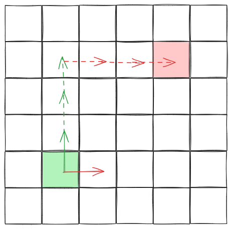
Here, the vector from the green square to the red square was written as

\[\mathbf{x} = 3\mathbf{e_1} + 3\mathbf{e_2}\]

as we needed 3 copies of the red vector (\(\mathbf{e_1}\)) and 3 of the green one (\(\mathbf{e_2}\)) to reach the red square from the green one.

But, in the same article we also considered another basis:

In this case, the same vector \(x\) was written as

\[\mathbf{x} = \mathbf{e_1'} + 2\mathbf{e_2'}\]

Where \(\mathbf{e_1'}\) was the orange vector and \(\mathbf{e_2'}\) was the blue one.

We did the same for the hexagonal grid and then concluded the article with the procedure to convert from one basis to another: represent each vector of the new base as a linear combination of the vectors forming the old basis.

Now, we are abstracting this a little. Using the first image, let’s say we denote \(\mathbf{x}\) as this collection of 2 numbers:

\[\begin{pmatrix} 3\\ 3 \end{pmatrix}\]

As it was written as \(\mathbf{x} = 3\mathbf{e_1} + 3\mathbf{e_2}\) in the first representation. Similarly, in the second representation, we can assign it this collection of numbers:

\[\begin{pmatrix} 1\\ 2 \end{pmatrix}\]

Is this sound? We can represent each basis vector as a column that has \(0\)s everywhere except in one position, and that position is \(1\). Then, any other linear combination of these vectors will be represented as the column that gives the corresponding coefficients. We can prove that this matches the two requirements for a vector space:

• multiplying with a scalar:

\[\alpha\begin{pmatrix}0\\\vdots\\0\\1\\0\\\vdots\\0\end{pmatrix}=\begin{pmatrix}0\\\vdots\\0\\\alpha\\0\\\vdots\\0\end{pmatrix}\]

• adding two vectors

\[\begin{pmatrix}a\\\vdots\\b\end{pmatrix}+\begin{pmatrix}c\\\vdots\\d\end{pmatrix}=\begin{pmatrix}a+c\\\vdots\\b+d\end{pmatrix}\]

What is left is to determine how to convert these column representations from one basis to another.

Looking back at the two images, we can write

\[\begin{matrix} \mathbf{e_1}' & = & \mathbf{e_1} & - & \mathbf{e_2}\\ \mathbf{e_2}' & = & \mathbf{e_1} & + & 2\mathbf{e_2} \end{matrix}\]

That is, in the first basis, \(\mathbf{e_1}'\) is identified to be the same as \(\begin{pmatrix}1\\-1\end{pmatrix}\), and \(\mathbf{e_2'}\) as \(\begin{pmatrix}1\\2\end{pmatrix}\). What happens if we just concatenate these two? We get this table, called a matrix:

\[A = \begin{pmatrix} 1 & 1 \\ -1 & 2 \end{pmatrix}\]

Now, let’s think of \(x\) represented in the second base by

\[\mathbf{x} = \mathbf{e_1'} + 2\mathbf{e_2'}\]

Let’s use the column representations for \(\mathbf{e_1'}\) and \(\mathbf{e_2'}\) in the non-prime base. Rewriting the above we have:

\[\mathbf{x} = 1 \begin{pmatrix}1\\-1\end{pmatrix} + 2\begin{pmatrix}1\\2\end{pmatrix}\]

But, this is one copy of the first column of \(A\) added to two copies of the second column! We can define matrix-vector multiplication as doing a linear combination of the columns of the matrix and then this last expression becomes

\[\mathbf{x} = A \begin{pmatrix}1\\2\end{pmatrix}\]

But wait! On the right side we \(\mathbf{x}\) written in terms of the original base, whereas on the left side everything is in term of the second one. That is:

\[\begin{pmatrix}3\\3\end{pmatrix} = \begin{pmatrix} 1 & 1 \\ -1 & 2 \end{pmatrix} \begin{pmatrix}1\\2\end{pmatrix}\]

Thi is why matrix multiplication is defined the way it is! It is just a simple linear combination of conversions from one vector basis to another one.

You can convince yourself that this is the case too, by looking at the hexagonal grid example from the previous article. As a spoiler, you should get to something like

\[\begin{pmatrix}3\\4\end{pmatrix} = \begin{pmatrix} 1 & 1 \\ 0 & 1 \end{pmatrix} \begin{pmatrix}-1\\4\end{pmatrix}\]

Thus, the essence of linear algebra is matrix multiplication, because this allows us to abstract away from the space where we define the vectors (like in these sets of articles we used square and hexagonal grids), and treat them all in the same way. Next article in the series will look at what the different ways to manipulate the matrices mean, grounded on the same 2 types of grids.